Compression: Nominal

Simulation

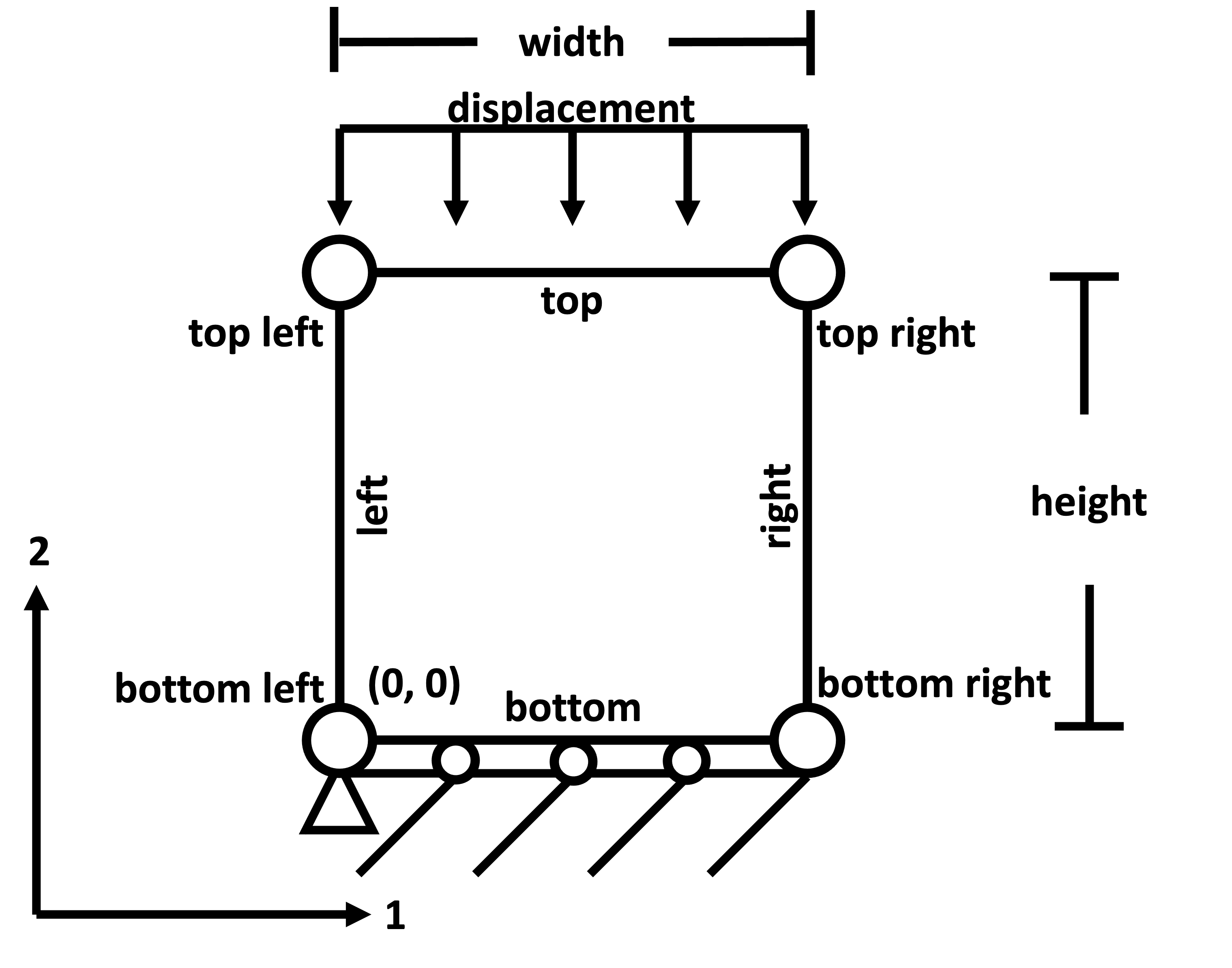
The rectangle model is simple demonstration for how to exercise the capabilities of a WAVES workflow [2]. It is a single 2D square, plane-stress element oriented in the 1-2 plane consisting of a mock, linear-elastic material model, simple boundary conditions, and applied uniaxial compression. The simulation preparation and solve are conducted in Abaqus [3].

Simulation schematic

The rectangle model is comprised of a single 2D square part with nominal dimensions 1mm x 1mm, but which can be parameterized by width and height by the journal file: modsim_package.abaqus.rectangle_geometry.

The bottom left node of the geometry is restricted in all six translational/rotational degrees of freedom using an encastre boundary condition. The bottom edge uses a roller boundary condition, with no translation in the 2 direction, but is free to move in the 1 direction.

Loading is prescribed as a uniaxial displacement of the top edge of the part in the negative 2 direction (compression), with a nominal displacement of -0.01 mm, which can be parameterized in the workflow.

A continuum plain stress (CPS4) element type is used for the rectangle model. The nominal mesh is 1 element for the square geometry, but this can be parameterized by the journal file modsim_package.abaqus.rectangle_mesh. More about Abaqus continuum elements can be found in the Abaqus documentation section titled “Solid Continuum Elements” [3].

A mock material definition was developed using the following parameters in the mmNsK unit system:

Material Parameters

Parameter name	Value	Units
Density	2.7E-09	\([Mg/mm^3]\)
Elastic Modulus	100	\([MPa]\)
Poisson’s Ratio	0.3	\([-]\)
Specific Heat	8.96E08	\([mJ/(MgK)]\)
Conductivity	132	\([mW/(mmK)]\)
Thermal Expansion	23.58E-6	\([1/K]\)

Theory

For an isotropic, homogeneous solid under plane stress conditions at constant temperature, as assumed in the simulation problem description, the constitutive model for stress and strain is given by the equations [4]

\[\sigma_{33} = \sigma_{23} = \sigma_{13} = 0\]

\[ \begin{align}\begin{aligned}\sigma_{11} = \frac{E}{1 - \nu^{2}} \left ( \epsilon_{11} + \nu\epsilon_{22} \right )\\\sigma_{22} = \frac{E}{1 - \nu^{2}} \left ( \epsilon_{22} + \nu\epsilon_{11} \right )\end{aligned}\end{align} \]

In the case of unconstrained transverse expansion, the transverse stress \(\sigma_{11}\) is zero and the theoretical expected stress in the direction of the applied displacement, \(\sigma_{22}\) is given by

\[\sigma_{22} = E \epsilon_{22}\]

With the material parameters from the Material Parameters Table and an applied strain of

\[\epsilon_{22} = \delta / L = -0.01 mm / 1.0 mm = -0.01 mm/mm\]

where \(L\) is the nominal starting height and \(\delta\) is the change in height, the expected stress for this simulation is

\[\sigma_{22} = E \epsilon_{22} = \left ( 100 MPa \right ) \left ( -0.01 mm/mm \right ) = -1 MPa\]

Results

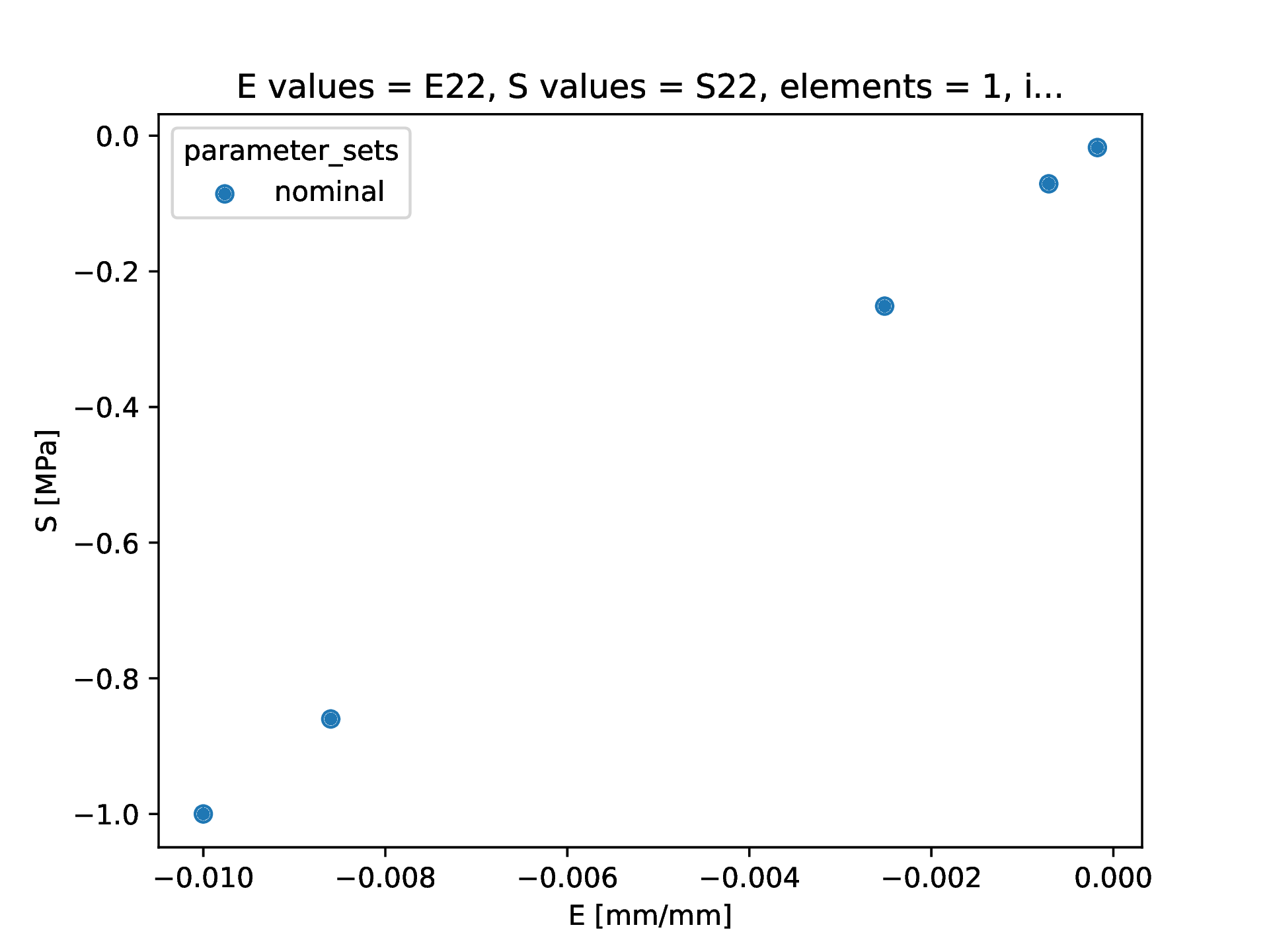
Stress-strain

Conclusions

The stress-strain plot shows that the simulation model is acting as expected with a linear elastic response through a 10% compressive strain load. This verifies that the geometry journal file and linear elastic material model are implemented correctly and provides confidence in the journal file and simulation input files for future simulations and analysis.