Constitutive Equations

Micromorphic Linear Elasticity

Eringen and Suhubi [3] proposed unique sets of elastic deformation measures as functions of the macroscopic deformation gradient \(\mathbf{F}\) and the micro-deformation tensor \(\mathbf{\chi}\). These deformation measures include the left Cauchy-Green deformation tensor \(\mathbf{\mathcal{C}}\), a tensor including both macro- and micro-deformations \(\mathbf{\Psi}\), and the micro-deformation gradient \(\mathbf{\Gamma}\), as calculated in Eq. (27). From the deformation measures introduced in Eq. (27), two strain measures are defined: the Green-Lagrange strain, \(\mathbf{E}\), and the micro-strain, \(\mathbf{\mathcal{E}}\), calculated according to equations (28) and (29), respectively.

A quadratic form for the Helmholtz free energy is introduced in equation (59) using \(\mathbf{E}\), \(\mathbf{\mathcal{E}}\), and \(\mathbf{\Gamma}\),

(59)\[ \begin{align}\begin{aligned}\left(\rho_{0}\psi\right)^e &= \frac{1}{2}E_{KL}A_{KLMN}E_{MN} + \frac{1}{2}\mathcal{E}_{KL}B_{KLMN}\mathcal{E}_{MN}\\&+ \frac{1}{2}\Gamma_{KLM}C_{KLMNPQ}\Gamma_{NPQ} + E_{KL}D_{KLMN}\mathcal{E}_{MN},\end{aligned}\end{align} \]

where \(\mathbf{A}\), \(\mathbf{B}\), \(\mathbf{C}\), and \(\mathbf{D}\) are the elastic material moduli tensors, which may be calculated according to equations (60), (61), (62), and (63), respectively.

(60)\[A_{KLMN} = \lambda\delta_{KL}\delta_{MN} + \mu \left(\delta_{KM}\delta_{LN} + \delta_{KN}\delta_{LM} \right)\]

(61)\[B_{KLMN} = \left(\eta - \tau\right) \delta_{KL}\delta_{MN} + \left(\kappa - \sigma\right) \delta_{KM}\delta_{LN} + \left(\nu - \sigma \right) \delta_{KN}\delta_{LM}\]

(62)\[ \begin{align}\begin{aligned}C_{LMKNPQ} &= \tau_1 \left(\delta_{LM}\delta_{KN}\delta_{PQ} + \delta_{LQ}\delta_{MK}\delta_{NP}\right) + \tau_2 \left(\delta_{LM}\delta_{KP}\delta_{NQ} + \delta_{LK}\delta_{MQ}\delta_{NP}\right)\\&+ \tau_3 \delta_{LM}\delta_{KQ}\delta_{NP} + \tau_4 \delta_{LN}\delta_{MK}\delta_{PQ} + \tau_5 \left(\delta_{LK}\delta_{MN}\delta_{PQ} + \delta_{LP}\delta_{MK}\delta_{NQ}\right)\\&+ \tau_6 \delta_{LK}\delta_{MP}\delta_{NQ} + \tau_7 \delta_{LN}\delta_{MP}\delta_{KQ} + \tau_8 \left(\delta_{LP}\delta_{MQ}\delta_{KN} + \delta_{LQ}\delta_{MN}\delta_{KP}\right)\\&+ \tau_9 \delta_{LN}\delta_{MQ}\delta_{KP} + \tau_10 \delta_{LP}\delta_{MN}\delta_{KQ} + \tau_{11} \delta_{LQ}\delta_{MP}\delta_{KN}\end{aligned}\end{align} \]

(63)\[D_{KLMN} = \tau\delta_{KL}\delta_{MN} + \sigma \left(\delta_{KN}\delta_{LM} + \delta_{LN}\delta_{KM}\right)\]

Equations (60), (61), (62), and (63) introduce the 18 parameters for the linear elastic micromorphic constitutive model. Calibration will seek to determine an admissible set of parameters that best describes the homogenized DNS response. The 18 parameters are identified as \(\lambda\), \(\mu\), \(\eta\), \(\tau\), \(\kappa\), \(\nu\), \(\sigma\), and \(\tau_{1}\) through \(\tau_{11}\). It should be noted that parameters \(\tau_{1}\) through \(\tau_{11}\) are only present in equation (62) which will be used to relate the micro-deformation gradient \(\mathbf{\Gamma}\) to higher order stress effects.

The stresses (second Piola-Kirchhoff stress \(\mathbf{S}\), symmetric micro-stress \(\mathbf{\Sigma}\), and higher order stress \(\mathbf{M}\)) may be derived from the Helmholtz free energy as follows:

(64)\[S_{IK} = 2 \frac{\partial\left(\rho_{0}\psi\right)^e}{\partial \mathcal{C}_{IJ}} + \frac{\partial\left(\rho_{0}\psi\right)^e}{\partial \Psi_{IQ}} \Psi_{KQ} \mathcal{C}_{JK}^{-1} + \frac{\partial\left(\rho_{0}\psi\right)^e}{\partial \Gamma_{IQK}} \Gamma_{SQK} \mathcal{C}_{JS}^{-1}\]

(65)\[\Sigma_{IJ} = 2 \frac{\partial\left(\rho_{0}\psi\right)^e}{\partial \mathcal{C}_{IJ}} + 2 symm\left[ \frac{\partial\left(\rho_{0}\psi\right)^e}{\partial \Psi_{IQ}} \Psi_{KQ} \mathcal{C}_{JK}^{-1} + \frac{\partial\left(\rho_{0}\psi\right)^e}{\partial \Gamma_{IQK}} \Gamma_{SQK} \mathcal{C}_{JS}^{-1} \right]\]

(66)\[M_{IJK} = \frac{\partial\left(\rho_{0}\psi\right)^e}{\partial \Gamma_{JKI}}.\]

By taking the relevant partial derivatives of the elastic Helmholtz free energy function, equations (64), (65), and (66) may be evaluated as follows:

(67)\[ \begin{align}\begin{aligned}S_{IJ} =& A_{IJKL}E_{KL} + D_{IJKL} \mathcal{E}_{KL} + \left\{B_{IQKL}\mathcal{E}_{KL} + E_{KL}D_{KLIQ}\right\}\left(\mathcal{E}_{RQ} + \delta_{RQ}\right) \left(\mathcal{C}_{RJ}\right)^{-1}\\&+ C_{IQRLMN} \Gamma_{LMN} \left(\mathcal{C}_{SJ}\right)^{-1} \Gamma_{SQR}\end{aligned}\end{align} \]

(68)\[ \begin{align}\begin{aligned}\Sigma_{IJ} =& A_{IJKL}E_{KL} + D_{IJKL} \mathcal{E}_{KL}\\&+ 2symm \left( \left\{B_{IQKL} \mathcal{E}_{KL} + E_{KL} D_{KLIQ} \right\} \left( \mathcal{E}_{RQ} + \delta_{RQ}\right) \left(\mathcal{C}_{RJ}\right)^{-1}\right)\\&+ 2symm \left(C_{IQRLMN} \Gamma_{LMN} \Gamma_{SQR} \left(\mathcal{C}_{SJ}\right)^{-1} \right)\end{aligned}\end{align} \]

(69)\[M_{IJK} = C_{JKILMN} \Gamma_{LMN}.\]

The above equations describe the full form of micromorphic linear elasticity.

For a simplified description of the linear elasticity model as a function of the 18 elasticity parameters, one may assume that elastic strains are small (but rotations may be large) and quadratic terms ignored. The second and third order stresses may be defined as follows:

(70)\[S_{IJ} = \left(\lambda^* + \tau^*\right) E_{MM} \delta_{IJ} + 2\left(\mu^* + \sigma^*\right) E_{IJ} + \eta^* \mathcal{E}_{MM} \delta_{IJ} + \kappa^* \mathcal{E}_{IJ} + \nu^* \mathcal{E}_{JI}\]

(71)\[ \begin{align}\begin{aligned}\Sigma_{IJ} &= \left(\lambda^* + 2\tau^*\right) E_{MM} \delta_{IJ} + 2\left(\mu^* + 2\sigma^*\right) E_{IJ} + \left(2\eta^* - \tau^*\right) \mathcal{E}_{MM} \delta_{IJ}\\&+ \left(\nu^* + \kappa^* - \sigma\right) \left(\mathcal{E}_{IJ} + \mathcal{E}_{JI}\right)\end{aligned}\end{align} \]

(72)\[ \begin{align}\begin{aligned}M_{IJK} &= \tau_1^* \left(\delta_{JK}\Gamma_{IPP} + \delta_{KI} \Gamma_{PPJ}\right) + \tau_2^* \left(\delta_{JK}\Gamma_{NIN} + \delta_{JI} \Gamma_{PPK}\right)\\&+ \tau_3^* \delta_{JK} \Gamma_{NNI} + \tau_4^* \delta_{KI} \Gamma_{JPP} + \tau_5^* \left(\delta_{JI}\Gamma_{KPP} + \delta_{KI} \Gamma_{NJN}\right)\\&+ \tau_6^* \delta_{JI} \Gamma_{NKN} + \tau_7^* \Gamma_{JKI} + \tau_8^* \left(\Gamma_{IJK} + \Gamma_{KIJ}\right) + \tau_9^* \Gamma_{JIK}\\ &+ \tau_{10}^* \Gamma_{KJI} + \tau_{11}^* \Gamma_{IJK},\end{aligned}\end{align} \]

which are the same as shown in equation (4) (although here different indices are used) discussed in the Micromorphic Linear Elasticity section while describing the micromorphic upscaling workflow. It should be noted that no aspects of the Tardigrade toolchain (including the material point calibration library and Tardigrade-MOOSE) make use of these assumptions, however, these equations simplify the discussion and are more conceptually intuitive.

Smith Conditions

Refer to the Constraints on Elastic Parameters section for the discussion of the Smith conditions.

Micromorphic Elasto-plasticity

Kinematics

A multiplicative decomposition of the macro deformation gradient and micro deformation tensor is used to separate elastic and plastic effects.

\[ \begin{align}\begin{aligned}F_{iI} &= F^{e}_{i\bar{I}} F^p_{\bar{I}I}\\\chi_{iI} &= \chi^{e}_{i\bar{I}} \chi^p_{\bar{I}I}\end{aligned}\end{align} \]

Figure 51 (borrowed from Miller 2021 [1] Figure 3.1) shows the effect of the multiplicative decomposition and resulting configuration spaces. As before, the reference configuration maps to the current configuration through \(\mathbf{F}\) and \(\mathbf{\chi}\). A stress free, intermediate configuration (\(\bar{B}\)) is introduced which maps from the reference configuration through \(\mathbf{F^p}\) and \(\mathbf{\chi^p}\). The overbar notation \(\bar{.}\) denotes quantities in the intermediate configuration. Figure 51 show the independent actions of macro deformation gradients and micro deformation tensors.

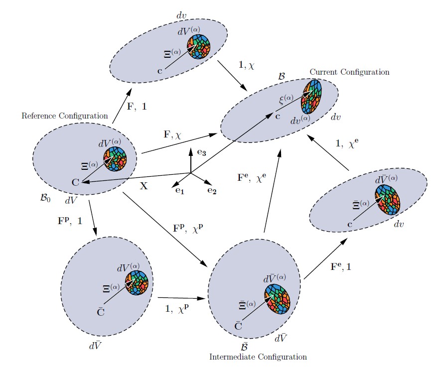
Fig. 51 Configuration spaces of the multiplicative decomposition of \(\mathbf{F}\) and \(\mathbf{\chi}\)

The elastic deformation measures from equations (27), (28), and (29) are now defined in the intermediate configuration as

(73)\[ \begin{align}\begin{aligned}\bar{\mathcal{C}}^e_{\bar{I}\bar{J}} &= F^e_{i\bar{I}} F^e_{i\bar{J}}\\\bar{\Psi}^e_{\bar{I}\bar{J}} &= F^e_{i\bar{I}} \chi^e_{i\bar{J}}\\\bar{\Gamma}^e_{\bar{I}\bar{J}K} &= F^e_{i\bar{I}} \chi^e_{i\bar{J},\bar{K}}\\\bar{E}^e_{\bar{I}\bar{J}} &= \frac{1}{2} \left( \mathcal{C}^e_{\bar{I}\bar{J}} - \delta_{\bar{I}\bar{J}} \right)\\\bar{\mathcal{E}}^e_{\bar{I}\bar{J}} &= \Psi^e_{\bar{I}\bar{J}} - \delta_{\bar{I}\bar{J}}\end{aligned}\end{align} \]

Further details of micromorphic elastoplasticity may be found in Chapter 3 of Miller 2021 [1].

Deviatoric Stress Measures

The deviatoric parts of the Cauchy, symmetric micro-, and higher-order stresses may be defined in the current configuration as

\[ \begin{align}\begin{aligned}dev\left(\sigma_{ij}\right) & \stackrel{\text{def}}{=} \sigma_{ij} - \frac{1}{3}\sigma_{kk}\delta_{ij}\\dev\left(s_{ij}\right) & \stackrel{\text{def}}{=} s_{ij} - \frac{1}{3} s_{kk}\delta_{ij}\\dev\left(m_{ijk}\right) & \stackrel{\text{def}}{=} m_{ijk} - \frac{1}{3} m_{llk}\delta_{ij}.\end{aligned}\end{align} \]

The Cauchy, micro-, and higher-order pressures may be defined in the current configuration as

\[ \begin{align}\begin{aligned}p^u &\stackrel{\text{def}}{=} \frac{1}{3}\sigma_{kk} = \frac{1}{3 J^e} F^e_{i\bar{I}}\bar{S}_{\bar{I}\bar{J}}F^e_{i\bar{J}} = \frac{1}{3 J^e}\bar{C}^e_{\bar{I}\bar{J}}\bar{S}_{\bar{I}\bar{J}}\\p^{\chi} &= \frac{1}{3} s_{kk} = \frac{1}{3 J^e}\bar{C}^e_{\bar{I}\bar{J}}\bar{\Sigma}_{\bar{I}\bar{J}}\\p^{\nabla\chi}_k &= \frac{1}{3} m_{llk} = \frac{1}{3 J^e}\bar{M}_{\bar{I}\bar{J}\bar{K}}\bar{C}^e_{\bar{I}\bar{J}}\chi^e_{k\bar{K}}\end{aligned}\end{align} \]

where \(\bar{C}^e_{\bar{I}\bar{J}}=F^e_{i\bar{I}}F^e_{j\bar{J}}\). These pressures may be defined in the intermediate configuration as

\[ \begin{align}\begin{aligned}\bar{p}^u & =\frac{1}{3}\bar{C}^e_{\bar{I}\bar{J}}\bar{S}_{\bar{I}\bar{J}}\\\bar{p}^{\chi} &=\frac{1}{3}\bar{C}^e_{\bar{I}\bar{J}}\bar{\Sigma}_{\bar{I}\bar{J}}\\\bar{p}^{\nabla\chi}_{\bar{K}} &= \frac{1}{3}\bar{C}^e_{\bar{I}\bar{J}}\bar{M}_{\bar{I}\bar{J}\bar{K}}.\end{aligned}\end{align} \]

Using these terms, the deviatoric parts of the Second Piola-Kirchhoff, symmetric micro- and higher-order stresses may be written in the intermediate configuration as

\[ \begin{align}\begin{aligned}dev\left(\bar{S}_{\bar{I}\bar{J}}\right) &= \bar{S}_{\bar{I}\bar{J}} - \bar{p}^u\left(\bar{C}^e_{\bar{I}\bar{J}}\right)^{-1}\\dev\left(\bar{\Sigma}_{\bar{I}\bar{J}}\right) &= \bar{\Sigma}_{\bar{I}\bar{J}} - \bar{p}^{\chi}\left(\bar{C}^e_{\bar{I}\bar{J}}\right)^{-1}\\dev\left(\bar{M}_{\bar{I}\bar{J}\bar{K}}\right) &= \bar{M}_{\bar{I}\bar{J}\bar{K}} - \bar{p}_{\bar{K}}^{\nabla\chi}\left(\bar{C}^e_{\bar{I}\bar{J}}\right)^{-1}.\end{aligned}\end{align} \]

Helmholtz Free Energy Function

A micromorphic, linear isotropic, Drucker-Prager elastoplasticity is considered. The total Helmholtz free energy per unit mass in the intermediate configuration may be expressed as the addition of the elastic free energy function \(\left( \bar{\rho} \bar{\psi}\right)^e\) (introduced in Eq. (59) in the reference configuration) and plastic free energy function \(\left( \bar{\rho} \bar{\psi}\right)^p\).

\[\left(\bar{\rho} \bar{\psi}\right) \stackrel{\text{def}}{=} \left(\bar{\rho} \bar{\psi}\right)^e + \left(\bar{\rho} \bar{\psi}\right)^p\]

A quadratic form of the plastic Helmholtz energy function is defined as a function of strain-like internal state variables (ISVs) and hardening moduli.

(74)\[\left(\bar{\rho} \bar{\psi}\right)^p \stackrel{\text{def}}{=} \frac{1}{2}\bar{H}^u \left(\bar{Z}^u\right)^2 + \frac{1}{2}\bar{H}^{\chi} \left(\bar{Z}^{\chi}\right)^2 + \frac{1}{2}\bar{Z}^{\chi}_{,\bar{I}} \bar{H}_{\bar{I}\bar{J}}^{\nabla\chi} \bar{Z}^{\chi}_{,\bar{J}}\]

where \(\bar{Z}^u\) and \(\bar{Z}^{\chi}\) are scalars.

As will be discussed in the proceeding section, Yield Surfaces, three yield surfaces are defined for macro- (\(u\)), micro- (\(\chi\)), and micro-gradient plasticity (\(\nabla\chi\)) with associated strain-like ISVs (\(\bar{Z}^u\), \(\bar{Z}^{\chi}\), and \(\bar{Z}^{\nabla \chi}\)) and hardening moduli (\(\bar{H}^u\), \(\bar{H}^{\chi}\), and \(\bar{H}^{\nabla \chi}\)). Stress-like ISVs are defined as

(75)\[ \begin{align}\begin{aligned}\bar{Q}^u &\stackrel{\text{def}}{=} \frac{\partial \left( \bar{\rho} \bar{\psi} \right)}{\partial \bar{Z}^u_{\bar{I}}} = \bar{H}^u\bar{Z}^u\\\bar{Q}^{\chi} &\stackrel{\text{def}}{=} \frac{\partial \left( \bar{\rho} \bar{\psi} \right)}{\partial \bar{Z}^{\chi}_{\bar{I}}} = \bar{H}^{\chi}\bar{Z}^{\chi}\\\bar{Q}^{\nabla\chi}_{\bar{I}} &\stackrel{\text{def}}{=} \frac{\partial \left( \bar{\rho} \bar{\psi} \right)}{\partial \bar{Z}^{\nabla\chi}_{\bar{I},\bar{J}}} = \bar{H}^{\nabla\chi}_{\bar{I}\bar{J}}\bar{Z}^{\chi}_{,\bar{J}}.\end{aligned}\end{align} \]

For isotropy, the micro-gradient hardening moduli are simplified to \(\bar{H}^{\nabla\chi}_{\bar{I}\bar{J}}=\bar{H}^{\nabla\chi} \delta_{\bar{I}\bar{J}}\) which reduces the stress-like ISV to \(\bar{Q}^{\chi}_{\bar{I}}=\bar{H}^{\nabla\chi}\bar{Z}^{\chi}_{,\bar{I}}\).

Yield Surfaces

The Drucker-Prager yield functions may be defined for macro- (\(u\)), micro- (\(\chi\)), and micro-gradient plasticity (\(\nabla\chi\)) as

\[ \begin{align}\begin{aligned}\bar{F}^u\left(\bar{\mathbf{S}},\bar{c}^u\right) &\stackrel{\text{def}}{=} ||dev\left(\bar{\mathbf{S}}\right)|| - \left(A^{u,\phi}\bar{c}^u - B^{u,\phi} \bar{p}^u\right) \leq 0\\\bar{F}^{\chi}\left(\bar{\mathbf{\Sigma}},\bar{c}^{\chi}\right) &\stackrel{\text{def}}{=} ||dev\left(\bar{\mathbf{\Sigma}}\right)|| - \left(A^{{\chi},\phi}\bar{c}^{\chi} - B^{{\chi},\phi} \bar{p}^{\chi}\right) \leq 0\\\bar{F}_{\bar{K}}^{\nabla\chi}\left(\bar{\mathbf{M}},\bar{\mathbf{c}}^{\nabla\chi}\right) &\stackrel{\text{def}}{=} ||dev\left(\bar{\mathbf{M}}\right)||_{\bar{K}} - \left(A^{{\nabla\chi},\phi}\bar{c}_{\bar{K}}^{\nabla\chi} - B^{{\nabla\chi},\phi} \bar{p}_{\bar{K}}^{\nabla\chi}\right) \leq 0\end{aligned}\end{align} \]

where \(\bar{c}^u\), \(\bar{c}^{\chi}\), and \(\bar{c}^{\nabla\chi}\) are the cohesion terms for each of the respective yield surface. Note that there are 3 yield surface for micro-gradient plasticity. The invariants of the stress measures are defined as

\[ \begin{align}\begin{aligned}||dev\left(\bar{\mathbf{S}}\right)|| &= \sqrt{\left(dev \left( \bar{S}_{\bar{I}\bar{J}}\right)\right) : \left(dev \left(\bar{S}_{\bar{I}\bar{J}}\right) \right)}\\||dev\left(\bar{\mathbf{\Sigma}}\right)|| &= \sqrt{\left(dev \left( \bar{\Sigma}_{\bar{I}\bar{J}}\right) \right) : \left(dev \left(\bar{\Sigma}_{\bar{I}\bar{J}}\right) \right)}\\||dev\left(\bar{\mathbf{M}}\right)||_{\bar{K}} &= \sqrt{\left(dev \left( \bar{M}_{\bar{I}\bar{J}\left(\bar{K}\right)}\right) \right) : \left(dev \left(\bar{M}_{\bar{I}\bar{J}\left(\bar{K}\right)}\right) \right)}.\end{aligned}\end{align} \]

The notation \(\left(\bar{K}\right)\) indicates that the \(\bar{K}\) index is free so \(||dev\left(\bar{\mathbf{M}}\right)||_{\bar{K}}\) represents a vector of invariants of the higher-order stress. These yield functions depend on the friction angles (\(\phi^u\), \(\phi^{\chi}\), and \(\phi^{\nabla\chi}\)) through the functions

(76)\[ \begin{align}\begin{aligned}&A^{u,\phi}=\beta^{u,\phi}\cos\left(\phi^u\right) , B^{u,\phi}=\beta^{u,\phi}\sin\left(\phi^u\right) , \beta^{u,\phi} = \frac{2\sqrt{6}}{3+\tilde{\beta}^{u,\phi} \sin\left(\phi^u\right)}\\&A^{{\chi},\phi}=\beta^{{\chi},\phi}\cos\left(\phi^{\chi}\right) , B^{{\chi},\phi}=\beta^{{\chi},\phi}\sin\left(\phi^{\chi}\right) , \beta^{{\chi},\phi} = \frac{2\sqrt{6}}{3+\tilde{\beta}^{\chi,\phi} \sin\left(\phi^{\chi}\right)}\\&A^{{\nabla\chi},\phi}=\beta^{{\nabla\chi},\phi}\cos\left(\phi^{\nabla\chi}\right) , B^{{\nabla\chi},\phi}=\beta^{{\nabla\chi},\phi}\sin\left(\phi^{\nabla\chi}\right) , \beta^{{\nabla\chi},\phi} = \frac{2\sqrt{6}}{3+\tilde{\beta}^{\nabla\chi,\phi} \sin\left(\phi^{\nabla\chi}\right)}.\end{aligned}\end{align} \]

The parameters \(\tilde{\beta}^{u,\phi}\), \(\tilde{\beta}^{\chi,\phi}\), and \(\tilde{\beta}^{\nabla\chi,\phi}\) are parameters ranging from \(+/-\) 1 to control how the yield function relates to the Mohr-Coloumb yield surface. In a similar manner as the yield functions, the plastic potential functions for macro- (\(u\)), micro- (\(\chi\)), and micro-gradient plasticity (\(\nabla\chi\)) are defined as

(77)\[ \begin{align}\begin{aligned}\bar{G}^u\left(\bar{\mathbf{S}},\bar{c}^u\right) &\stackrel{\text{def}}{=} ||dev\left(\bar{\mathbf{S}}\right)|| - \left(A^{u,\psi}\bar{c}^u - B^{u,\psi} \bar{p}^u\right)\\\bar{G}^{\chi}\left(\bar{\mathbf{\Sigma}},\bar{c}^{\chi}\right) &\stackrel{\text{def}}{=} ||dev\left(\bar{\mathbf{\Sigma}}\right)|| - \left(A^{{\chi},\psi}\bar{c}^{\chi} - B^{{\chi},\psi} \bar{p}^{\chi}\right)\\\bar{G}_{\bar{K}}^{\nabla\chi}\left(\bar{\mathbf{M}},\bar{\mathbf{c}}^{\nabla\chi}\right) &\stackrel{\text{def}}{=} ||dev\left(\bar{\mathbf{M}}\right)||_{\bar{K}} - \left(A^{{\nabla\chi},\psi}\bar{c}_{\bar{K}}^{\nabla\chi} - B^{{\nabla\chi},\psi} \bar{p}_{\bar{K}}^{\nabla\chi}\right).\end{aligned}\end{align} \]

The plastic potential functions depend on the dilation angles (\(\psi^u\), \(\psi^{\chi}\), and \(\psi^{\nabla\chi}\)) through functions of identical form as shown in Eq. (76) except the \(\phi\) terms are replaced with \(\psi\). Similarly, parameters \(\tilde{\beta}^{u,\psi}\), \(\tilde{\beta}^{\chi,\psi}\), and \(\tilde{\beta}^{\nabla\chi,\psi}\) range from \(+/-\) 1 to control how the potential functions relate to the Mohr-Coloumb yield surface.

The evolution equations are presented in full detail in [1, 15]. For the present discussion, the evolution of the strain-like ISVs are

(78)\[ \begin{align}\begin{aligned}\dot{\bar{Z}}^u &= -\dot{\bar{\gamma}}^u \frac{\partial\bar{G}^u}{\partial\bar{c}^u} = A^{u,\psi} \dot{\bar{\gamma}}^u\\\dot{\bar{Z}}^{\chi} &= -\dot{\bar{\gamma}}^{\chi} \frac{\partial\bar{G}^{\chi}}{\partial\bar{c}^{\chi}} = A^{\chi,\psi} \dot{\bar{\gamma}}^{\chi}\\\dot{\bar{Z}}^{\chi}_{,\bar{I}} &= -\dot{\bar{\gamma}}^{\nabla\chi}_{\bar{J}} \frac{\partial\bar{G}^{\nabla\chi}_{\bar{J}}}{\partial\bar{c}^{\nabla\chi}_{\bar{I}}} = A^{\nabla\chi,\psi} \dot{\bar{\gamma}}^{\nabla\chi}_{\bar{J}}\delta_{\bar{I}\bar{J}}\end{aligned}\end{align} \]

where \(\dot{\bar{\gamma}}^u\), \(\dot{\bar{\gamma}}^{\chi}\), and \(\dot{\bar{\gamma}}^{\nabla\chi}_{\bar{J}}\) are plastic multipliers. We also introduce the evolution equations for the plastic deformation which arise from the dissipation inequality as

\[ \begin{align}\begin{aligned}\bar{H}_{\bar{I}\bar{J}}\left(\bar{\mathbf{S}}, \bar{\mathcal{Q}}\right) &\stackrel{\text{def}}{=} \dot{\bar{\gamma}} \frac{\partial \bar{G}}{\partial \bar{S}_{\bar{I}\bar{J}}}\\\bar{H}_{\bar{I}\bar{J}}^{\chi}\left(\bar{\mathbf{\Sigma}}, \bar{\mathcal{Q}}^{\chi}\right) &\stackrel{\text{def}}{=} \dot{\bar{\gamma}}^{\chi} \frac{\partial \bar{G}^{\chi}}{\partial \bar{\Sigma}_{\bar{I}\bar{J}}}\\\bar{H}_{\bar{I}\bar{J}\bar{K}}^{\nabla \chi}\left(\bar{\mathbf{M}}, \bar{\mathbf{\mathcal{Q}}}^{\nabla \chi}\right) &\stackrel{\text{def}}{=} \dot{\bar{\gamma}}^{\nabla \chi}_{\bar{L}} \frac{\partial \bar{G}^{\nabla\chi}_{\bar{L}}}{\partial \bar{M}_{\bar{I}\bar{J}\bar{K}}}\end{aligned}\end{align} \]

where

\[ \begin{align}\begin{aligned}\bar{H}_{\bar{I}\bar{J}}\left(\bar{\mathbf{S}}, \bar{\mathcal{Q}}\right) &\stackrel{\text{def}}{=} \bar{L}_{\bar{K}\bar{I}}^p \bar{C}_{\bar{K}\bar{J}}^{e} - \bar{\Psi}_{\bar{J}\bar{M}}^e \bar{L}_{\bar{M}\bar{N}}^{\chi,p} \chi_{\bar{N}k}^{e,-1} F_{k\bar{I}}^e\\\bar{H}_{\bar{I}\bar{J}}^{\chi}\left(\bar{\mathbf{\Sigma}}, \bar{\mathcal{Q}}^{\chi}\right) &\stackrel{\text{def}}{=} \bar{\Psi}_{\bar{J}\bar{M}}^e \bar{L}_{\bar{M}\bar{N}}^{\chi,p} \chi_{\bar{N}k}^{e,-1} F_{k\bar{I}}^e\\\bar{H}_{\bar{I}\bar{J}\bar{K}}^{\nabla \chi}\left(\bar{\mathbf{M}}, \bar{\mathbf{\mathcal{Q}}}^{\nabla \chi}\right) &\stackrel{\text{def}}{=} \left( \left( \chi_{j\bar{N},\bar{I}}^e \dot{\chi}_{\bar{N}I}^p + \chi_{j\bar{N}}^e \dot{\chi}_{\bar{N}I,\bar{I}}^p - \chi_{j\bar{N}}^e \bar{L}_{\bar{N}\bar{M}}^{\chi} \chi_{\bar{M}I,\bar{I}}^p \right) \chi_{I\bar{K}}^{p,-1} - \nu_{jm}^p \chi_{m\bar{K},\bar{I}}^{e} \right) F_{j\bar{J}}^e.\end{aligned}\end{align} \]

In this expression, \(\bar{\bf{L}}^p\) is the macro-plastic velocity gradient, \(\bar{\bf{L}}^{\chi,p}\) is the micro-plastic velocity gradient, \(\bar{\Psi}^e_{\bar{I}\bar{J}} = F_{i\bar{I}}^e \chi_{i\bar{J}}^e\), and \(\nu_{ij}^p = \chi_{i\bar{I}}^e \dot{\chi}_{\bar{I}I}^p \chi_{I\bar{J}}^{p,-1} \chi_{\bar{J}j}^e\). Finally, the cohesion terms will evolve as

(79)\[ \begin{align}\begin{aligned}\bar{c}^u &= \bar{H}^u\bar{Z}^u\\\bar{c}^{\chi} &= \bar{H}^{\chi}\bar{Z}^{\chi}\\\bar{c}^{\nabla\chi}_{\bar{I}} &=\bar{H}^{\nabla\chi}\bar{Z}^{\chi}_{,\bar{I}}\end{aligned}\end{align} \]

and initialize as

(80)\[ \begin{align}\begin{aligned}\bar{c}^u &= \bar{c}^{u,0} \text{ for } \bar{Z}^u = 0\\\bar{c}^{\chi} &= \bar{c}^{\chi, 0} \text{ for } \bar{Z}^{\chi} = 0\\\bar{c}^{\nabla\chi}_{\bar{I}} &=\bar{c}^{\nabla\chi,0} \overrightarrow{1} \text{ for } \bar{Z}^{\chi}_{,\bar{I}} = 0\end{aligned}\end{align} \]

where \(\overrightarrow{1}\) is a vector of ones. For this form of micromorphic elastoplasticity, a user must specify 18 parameters in addition to the 18 linear elasticity parameters:

• initial cohesion value: \(c^{u,0}\), \(c^{\chi,0}\), and \(c^{\nabla\chi,0}\)

• hardening (or softening if negative) moduli: \(\bar{H}^u\), \(\bar{H}^{\chi}\), and \(\bar{H}^{\nabla\chi}\)

• friction angles: \(\phi^u\), \(\phi^{\chi}\), and \(\phi^{\nabla\chi}\)

• yield \(\tilde{\beta}\) parameters: \(\tilde{\beta}^{u,\phi}\), \(\tilde{\beta}^{\chi,\phi}\), and \(\tilde{\beta}^{\nabla\chi,\phi}\)

• dilation angles: (\(\psi^u\), \(\psi^{\chi}\), and \(\psi^{\nabla\chi}\))

• flow potential \(\tilde{\beta}\) parameters: \(\tilde{\beta}^{u,\psi}\), \(\tilde{\beta}^{\chi,\psi}\), and \(\tilde{\beta}^{\nabla\chi,\psi}\)

Choosing separate definition of the yield and flow potential parameters allows for non-associative plasticity to be modeled.

This model may be simplified by setting all friction and dilation angles to zero resulting associative, pressure insensitive, hardening plasticity with yield functions in the form of

(81)\[ \begin{align}\begin{aligned}\bar{F}^u\left(\bar{\mathbf{S}},\bar{c}^u\right) = ||dev\left(\bar{\mathbf{S}}\right)|| - 2 \sqrt{\frac{2}{3}}\bar{c}^u - \leq 0\\\bar{F}^{\chi}\left(\bar{\mathbf{\Sigma}},\bar{c}^{\chi}\right) = ||dev\left(\bar{\mathbf{\Sigma}}\right)|| - 2 \sqrt{\frac{2}{3}}\bar{c}^{\chi} \leq 0\\\bar{F}_{\bar{K}}^{\nabla\chi}\left(\bar{\mathbf{M}},\bar{\mathbf{c}}^{\nabla\chi}\right)= ||dev\left(\bar{\mathbf{M}}\right)||_{\bar{K}} - 2 \sqrt{\frac{2}{3}}\bar{c}_{\bar{K}}^{\nabla\chi} \leq 0.\end{aligned}\end{align} \]