Tutorial 04: Simulation#
References#
Environment#
SCons and WAVES can be installed in a Conda environment with the Conda package manager. See the Conda installation and Conda environment management documentation for more details about using Conda.
Note
The SALib and numpy versions may not need to be this strict for most tutorials. However, Tutorial: Sensitivity Study uncovered some undocumented SALib version sensitivity to numpy surrounding the numpy v2 rollout.
Create the tutorials environment if it doesn’t exist
$ conda create --name waves-tutorial-env --channel conda-forge waves 'scons>=4.6' matplotlib pandas pyyaml xarray seaborn 'numpy>=2' 'salib>=1.5.1' pytest
PS > conda create --name waves-tutorial-env --channel conda-forge waves scons matplotlib pandas pyyaml xarray seaborn numpy salib pytest
Activate the environment
$ conda activate waves-tutorial-env
PS > conda activate waves-tutorial-env
Some tutorials require additional third-party software that is not available for the Conda package manager. This
software must be installed separately and either made available to SConstruct by modifying your system’s PATH or by
modifying the SConstruct search paths provided to the waves.scons_extensions.add_program() method.
Warning
STOP! Before continuing, check that the documentation version matches your installed package version.
You can find the documentation version in the upper-left corner of the webpage.
You can find the installed WAVES version with
waves --version.
If they don’t match, you can launch identically matched documentation with the WAVES Command-Line Utility
docs subcommand as waves docs.
Directory Structure#
Create and change to a new project root directory to house the tutorial files if you have not already done so. For example
$ mkdir -p ~/waves-tutorials
$ cd ~/waves-tutorials
$ pwd
/home/roppenheimer/waves-tutorials
PS > New-Item $HOME\waves-tutorials -ItemType "Directory"
PS > Set-Location $HOME\waves-tutorials
PS > Get-Location

Path
----
C:\Users\roppenheimer\waves-tutorials
Note
If you skipped any of the previous tutorials, run the following commands to create a copy of the necessary tutorial files.
$ pwd
/home/roppenheimer/waves-tutorials
$ waves fetch --overwrite --tutorial 3 && mv tutorial_03_solverprep_SConstruct SConstruct
WAVES fetch
Destination directory: '/home/roppenheimer/waves-tutorials'
PS > Get-Location

Path
----
C:\Users\roppenheimer\waves-tutorials

PS > waves fetch --overwrite --tutorial 3 && Move-Item tutorial_03_solverprep_SConstruct SConstruct -Force
WAVES fetch
Destination directory: 'C:\Users\roppenheimer\waves-tutorials'
Fetch the
tutorial_03_solverprep.sconsfile and create a new file namedtutorial_04_simulation.sconswith the WAVES Command-Line Utility fetch subcommand.
$ pwd
/home/roppenheimer/waves-tutorials
$ waves fetch --overwrite tutorials/tutorial_03_solverprep.scons && cp tutorial_03_solverprep.scons tutorial_04_simulation.scons
WAVES fetch
Destination directory: '/home/roppenheimer/waves-tutorials'
PS > Get-Location

Path
----
C:\Users\roppenheimer\waves-tutorials

PS > waves fetch --overwrite tutorials\tutorial_03_solverprep.scons && Copy-Item tutorial_03_solverprep.scons tutorial_04_simulation.scons
WAVES fetch
Destination directory: 'C:\Users\roppenheimer\waves-tutorials'
SConscript#
Note
There is a large section of lines in the SConscript file that are not included before the next section of code
shown here, as they are identical to those from Tutorial 03: SolverPrep. The diff of the SConscript
file at the end of the SConscript section will demonstrate this more clearly.
Add the highlighted section shown below to the
tutorial_04_simulation.sconsfile. This will initialize the datacheck list.
waves-tutorials/tutorial_04_simulation.scons
22# Collect the target nodes to build a concise alias for all targets
23workflow = []
24datacheck = []
25
26# Geometry
27workflow.extend(
28    env.AbaqusJournal(
29        target=["rectangle_geometry.cae", "rectangle_geometry.jnl"],
30        source=["#/modsim_package/abaqus/rectangle_geometry.py"],
31        subcommand_options="",
32    )
33)
Add the highlighted sections shown below to the
tutorial_04_simulation.sconsfile. This will create the datackeck alias.
waves-tutorials/tutorial_04_simulation.scons
126# Collector alias based on parent directory name
127env.Alias(workflow_name, workflow)
128env.Alias(f"{workflow_name}_datacheck", datacheck)
129
130if not env["unconditional_build"] and not env["ABAQUS_PROGRAM"]:
131    print(f"Program 'abaqus' was not found in construction environment. Ignoring '{workflow_name}' target(s)")
132    Ignore([".", workflow_name], workflow)
133    Ignore([".", f"{workflow_name}_datacheck"], datacheck)
Running a Datacheck#
Modify your
tutorial_04_simulation.sconsfile by adding the contents shown below immediately after the code pertaining to# SolverPrepfrom the previous tutorial.
waves-tutorials/tutorial_04_simulation.scons
 75# Abaqus Solve
 76solve_source_list = [
 77    "rectangle_compression.inp",
 78    "assembly.inp",
 79    "boundary.inp",
 80    "field_output.inp",
 81    "materials.inp",
 82    "parts.inp",
 83    "history_output.inp",
 84    "rectangle_mesh.inp",
 85]
 86
 87datacheck.extend(
 88    env.AbaqusSolver(
 89        target=[
 90            "rectangle_compression_DATACHECK.odb",
 91            "rectangle_compression_DATACHECK.dat",
 92            "rectangle_compression_DATACHECK.msg",
 93            "rectangle_compression_DATACHECK.com",
 94            "rectangle_compression_DATACHECK.prt",
 95            "rectangle_compression_DATACHECK.023",
 96            "rectangle_compression_DATACHECK.mdl",
 97            "rectangle_compression_DATACHECK.sim",
 98            "rectangle_compression_DATACHECK.stt",
 99        ],
100        source=solve_source_list,
101        job="rectangle_compression_DATACHECK",
102        program_options="-double both -datacheck",
103    )
104)
The solve_source_list variable looks similar to the solver prep list added in Tutorial 03: SolverPrep. There are
two important differences. First, the solve source list uses the file basenames. The solver prep task copied the
necessary Abaqus input files into the build directory. When we refer to the file basenames, SCons will know to look for
the copy in the current build directory. Second, the rectangle_mesh.inp file has been added to the end of the solve
source list. This is the mesh file produced by the mesh task defined in Tutorial 02: Partition and Mesh.
The code snippet will define an optional task called a datacheck. You can read the Abaqus Standard/Explicit
Execution documentation [42] for more details on running a datacheck. The primary purpose for running a
datacheck is to verify the input file construction without running a full simulation. While Abaqus can continue with an
analysis from the datacheck output, doing so modifies the datacheck output files, which has the affect of prompting
SCons to always re-build the datacheck target. This task is excluded from the main workflow to avoid duplicate
preprocessing of the input file. It will be used later in Tutorial 11: Regression Testing.
One new section of code that we have not utilized yet in the previous tutorials is the passing of command-line options
to the builder. This is done using the program_options variable. Here, we instruct the Abaqus solver to use double
precision for both the packager and the analysis. See the Abaqus Precision Level for Executables documentation
[42] for more information about the use of single or double precision in an Abaqus analysis.
The solve_source_list and target lists are hardcoded for clarity in the tutorials. Python users familiar with list
comprehensions and the pathlib module should be able to construct the solve_source_list from the
copy_source_list introduced in Tutorial 03: SolverPrep. Similarly, the datacheck target list could be constructed
from a list comprehension and Python f-strings.
Running the Analysis#
Modify your
tutorial_04_simulation.sconsfile by adding the contents below immediately after the Abaqus datacheck code that was just discussed.
waves-tutorials/tutorial_04_simulation.scons
108workflow.extend(
109    env.AbaqusSolver(
110        target=[
111            "rectangle_compression.odb",
112            "rectangle_compression.dat",
113            "rectangle_compression.msg",
114            "rectangle_compression.com",
115            "rectangle_compression.prt",
116            "rectangle_compression.sta",
117        ],
118        source=solve_source_list,
119        job="rectangle_compression",
120        program_options="-double both",
121    )
122)
The changes you just made will be used to define the task for running the rectangle_compression analysis.
The next step should now be quite familiar - we extend the workflow list to include that task for running the
simulation with the waves.scons_extensions.abaqus_solver_builder_factory() builder. The source list uses the
existing solve_source_list variable because the datacheck and solve tasks share the same dependencies. The job
task keyword argument has dropped the DATACHECK suffix. The -double both option is included with the
program_options variable.
The program_options are again hardcoded for clarity in the tutorials, but Python users may have identified this as
an opportunity to collect the common datacheck and solve task options in a common variable to ensure consistency in
Abaqus options.
In summary of the changes you just made to the tutorial_04_simulation.scons file, a diff against the SConscript
file from Tutorial 03: SolverPrep is included below to help identify the changes made in this tutorial. Note the
addition of a separate datacheck alias, which will be used in Tutorial 11: Regression Testing.
waves-tutorials/tutorial_04_simulation.scons
--- /home/runner/work/waves/waves/build/docs/tutorials_tutorial_03_solverprep.scons
+++ /home/runner/work/waves/waves/build/docs/tutorials_tutorial_04_simulation.scons
@@ -22,6 +22,7 @@

 # Collect the target nodes to build a concise alias for all targets
 workflow = []
+datacheck = []

 # Geometry
 workflow.extend(
@@ -72,9 +73,62 @@

 # Comment used in tutorial code snippets: marker-4

+# Abaqus Solve
+solve_source_list = [
+    "rectangle_compression.inp",
+    "assembly.inp",
+    "boundary.inp",
+    "field_output.inp",
+    "materials.inp",
+    "parts.inp",
+    "history_output.inp",
+    "rectangle_mesh.inp",
+]
+
+datacheck.extend(
+    env.AbaqusSolver(
+        target=[
+            "rectangle_compression_DATACHECK.odb",
+            "rectangle_compression_DATACHECK.dat",
+            "rectangle_compression_DATACHECK.msg",
+            "rectangle_compression_DATACHECK.com",
+            "rectangle_compression_DATACHECK.prt",
+            "rectangle_compression_DATACHECK.023",
+            "rectangle_compression_DATACHECK.mdl",
+            "rectangle_compression_DATACHECK.sim",
+            "rectangle_compression_DATACHECK.stt",
+        ],
+        source=solve_source_list,
+        job="rectangle_compression_DATACHECK",
+        program_options="-double both -datacheck",
+    )
+)
+
+# Comment used in tutorial code snippets: marker-5
+
+workflow.extend(
+    env.AbaqusSolver(
+        target=[
+            "rectangle_compression.odb",
+            "rectangle_compression.dat",
+            "rectangle_compression.msg",
+            "rectangle_compression.com",
+            "rectangle_compression.prt",
+            "rectangle_compression.sta",
+        ],
+        source=solve_source_list,
+        job="rectangle_compression",
+        program_options="-double both",
+    )
+)
+
+# Comment used in tutorial code snippets: marker-6
+
 # Collector alias based on parent directory name
 env.Alias(workflow_name, workflow)
+env.Alias(f"{workflow_name}_datacheck", datacheck)

 if not env["unconditional_build"] and not env["ABAQUS_PROGRAM"]:
     print(f"Program 'abaqus' was not found in construction environment. Ignoring '{workflow_name}' target(s)")
     Ignore([".", workflow_name], workflow)
+    Ignore([".", f"{workflow_name}_datacheck"], datacheck)
SConstruct#
Add
tutorial_04_simulationto theworkflow_configurationslist in theSConstructfile.
A diff against the SConstruct file from Tutorial 03: SolverPrep is included below to help identify the
changes made in this tutorial.
waves-tutorials/SConstruct
--- /home/runner/work/waves/waves/build/docs/tutorials_tutorial_03_solverprep_SConstruct
+++ /home/runner/work/waves/waves/build/docs/tutorials_tutorial_04_simulation_SConstruct
@@ -1,5 +1,5 @@
 #! /usr/bin/env python
-"""Configure the WAVES solver preparation tutorial."""
+"""Configure the WAVES simulation tutorial."""

 import os
 import pathlib
@@ -100,6 +100,7 @@
     "tutorial_01_geometry.scons",
     "tutorial_02_partition_mesh.scons",
     "tutorial_03_solverprep.scons",
+    "tutorial_04_simulation.scons",
 ]
 for workflow in workflow_configurations:
     build_dir = env["variant_dir_base"] / pathlib.Path(workflow).stem
Build Targets#
Build the new targets
$ pwd
/home/roppenheimer/waves-tutorials
$ scons tutorial_04_simulation
scons: Reading SConscript files ...
Checking whether '/apps/abaqus/Commands/abq2024' program exists.../apps/abaqus/Commands/abq2024
Checking whether '/usr/projects/ea/abaqus/Commands/abq2024' program exists...no
Checking whether 'abq2024' program exists.../apps/abaqus/Commands/abq2024
Checking whether 'abaqus' program exists...no
scons: done reading SConscript files.
scons: Building targets ...
cd /home/roppenheimer/waves-tutorials/build/tutorial_04_simulation && /apps/abaqus/Commands/abq2024 cae -noGui /home/roppenheimer/waves-tutorials/modsim_package/abaqus/rectangle_geometry.py -- > rectangle_geometry.stdout 2>&1
cd /home/roppenheimer/waves-tutorials/build/tutorial_04_simulation && /apps/abaqus/Commands/abq2024 cae -noGui /home/roppenheimer/waves-tutorials/modsim_package/abaqus/rectangle_partition.py -- > rectangle_partition.stdout 2>&1
cd /home/roppenheimer/waves-tutorials/build/tutorial_04_simulation && /apps/abaqus/Commands/abq2024 cae -noGui /home/roppenheimer/waves-tutorials/modsim_package/abaqus/rectangle_mesh.py -- > rectangle_mesh.stdout 2>&1
Copy("build/tutorial_04_simulation/rectangle_compression.inp", "modsim_package/abaqus/rectangle_compression.inp")
Copy("build/tutorial_04_simulation/assembly.inp", "modsim_package/abaqus/assembly.inp")
Copy("build/tutorial_04_simulation/boundary.inp", "modsim_package/abaqus/boundary.inp")
Copy("build/tutorial_04_simulation/field_output.inp", "modsim_package/abaqus/field_output.inp")
Copy("build/tutorial_04_simulation/materials.inp", "modsim_package/abaqus/materials.inp")
Copy("build/tutorial_04_simulation/parts.inp", "modsim_package/abaqus/parts.inp")
Copy("build/tutorial_04_simulation/history_output.inp", "modsim_package/abaqus/history_output.inp")
cd /home/roppenheimer/waves-tutorials/build/tutorial_04_simulation && /apps/abaqus/Commands/abq2024 -job rectangle_compression -input rectangle_compression -double both -interactive -ask_delete no > rectangle_compression.stdout 2>&1
scons: done building targets.
PS > Get-Location

Path
----
C:\Users\roppenheimer\waves-tutorials

PS > scons tutorial_04_simulation
scons: Reading SConscript files ...
Checking whether '/apps/abaqus/Commands/abq2024' program exists...no
Checking whether '/usr/projects/ea/abaqus/Commands/abq2024' program exists...no
Checking whether 'abq2024' program exists...C:\SIMULIA\Commands\abq2024.BAT
Checking whether 'abaqus' program exists...C:\SIMULIA\Commands\abaqus.BAT
scons: done reading SConscript files.
scons: Building targets ...
cd C:\Users\roppenheimer\waves-tutorials\build\tutorial_04_simulation && C:\SIMULIA\Commands\abq2024.BAT cae -noGUI C:\Users\roppenheimer\waves-tutorials\modsim_package\abaqus\rectangle_geometry.py -- > C:\Users\roppenheimer\waves-tutorials\build\tutorial_04_simulation\rectangle_geometry.cae.stdout 2>&1
cd C:\Users\roppenheimer\waves-tutorials\build\tutorial_04_simulation && C:\SIMULIA\Commands\abq2024.BAT cae -noGUI C:\Users\roppenheimer\waves-tutorials\modsim_package\abaqus\rectangle_partition.py -- > C:\Users\roppenheimer\waves-tutorials\build\tutorial_04_simulation\rectangle_partition.cae.stdout 2>&1
cd C:\Users\roppenheimer\waves-tutorials\build\tutorial_04_simulation && C:\SIMULIA\Commands\abq2024.BAT cae -noGUI C:\Users\roppenheimer\waves-tutorials\modsim_package\abaqus\rectangle_mesh.py -- > C:\Users\roppenheimer\waves-tutorials\build\tutorial_04_simulation\rectangle_mesh.inp.stdout 2>&1
Copy("build\tutorial_04_simulation\rectangle_compression.inp", "modsim_package\abaqus\rectangle_compression.inp")
Copy("build\tutorial_04_simulation\assembly.inp", "modsim_package\abaqus\assembly.inp")
Copy("build\tutorial_04_simulation\boundary.inp", "modsim_package\abaqus\boundary.inp")
Copy("build\tutorial_04_simulation\field_output.inp", "modsim_package\abaqus\field_output.inp")
Copy("build\tutorial_04_simulation\materials.inp", "modsim_package\abaqus\materials.inp")
Copy("build\tutorial_04_simulation\parts.inp", "modsim_package\abaqus\parts.inp")
Copy("build\tutorial_04_simulation\history_output.inp", "modsim_package\abaqus\history_output.inp")
cd C:\Users\roppenheimer\waves-tutorials\build\tutorial_04_simulation && C:\SIMULIA\Commands\abq2024.BAT -interactive -ask_delete no -job rectangle_compression -input rectangle_compression -double both > C:\Users\roppenheimer\waves-tutorials\build\tutorial_04_simulation\rectangle_compression.odb.stdout 2>&1
scons: done building targets.
Output Files#
Explore the contents of the build directory using the tree command against the build directory, as shown
below.
$ pwd
/home/roppenheimer/waves-tutorials
$ tree build/tutorial_04_simulation/
build/tutorial_04_simulation/
|-- abaqus.rpy
|-- abaqus.rpy.1
|-- abaqus.rpy.2
|-- assembly.inp
|-- boundary.inp
|-- field_output.inp
|-- history_output.inp
|-- materials.inp
|-- parts.inp
|-- rectangle_compression.com
|-- rectangle_compression.dat
|-- rectangle_compression.inp
|-- rectangle_compression.msg
|-- rectangle_compression.odb
|-- rectangle_compression.prt
|-- rectangle_compression.sta
|-- rectangle_compression.stdout
|-- rectangle_geometry.cae
|-- rectangle_geometry.cae.stdout
|-- rectangle_geometry.jnl
|-- rectangle_mesh.cae
|-- rectangle_mesh.inp
|-- rectangle_mesh.inp.stdout
|-- rectangle_mesh.jnl
|-- rectangle_partition.cae
|-- rectangle_partition.cae.stdout
`-- rectangle_partition.jnl

0 directories, 27 files
PS > Get-Location

   Path
   ----
   C:\Users\roppenheimer\waves-tutorials

PS > tree build\tutorial_04_simulation /F
C:\USERS\ROPPENHEIMER\WAVES-TUTORIALS\BUILD\TUTORIAL_04_SIMULATION
    abaqus.rpy
    abaqus.rpy.1
    abaqus.rpy.2
    assembly.inp
    boundary.inp
    field_output.inp
    history_output.inp
    materials.inp
    parts.inp
    rectangle_compression.com
    rectangle_compression.dat
    rectangle_compression.inp
    rectangle_compression.msg
    rectangle_compression.odb
    rectangle_compression.odb.stdout
    rectangle_compression.prt
    rectangle_compression.sta
    rectangle_geometry.cae
    rectangle_geometry.cae.stdout
    rectangle_geometry.jnl
    rectangle_mesh.cae
    rectangle_mesh.inp
    rectangle_mesh.inp.stdout
    rectangle_mesh.jnl
    rectangle_partition.cae
    rectangle_partition.cae.stdout
    rectangle_partition.jnl

No subfolders exist
The build/tutorial_04_simulation directory contains several different subsets of related files:
rectangle_{geometry,partition,mesh}.*- output files generated from the code pertaining to# Geometry,# Partition, and# Meshin theSConscriptfile. This code was first introduced in Tutorial 01: Geometry and Tutorial 02: Partition and Mesh, but it is important to note that each tutorial adds and executes a full workflow.*.inp- files copied to the build directory as part of the code pertaining to# SolverPrepin theSConscriptfile, which was introduced in Tutorial 03: SolverPrep.rectangle_compression.*- output files from Running the Analysis in this tutorial.
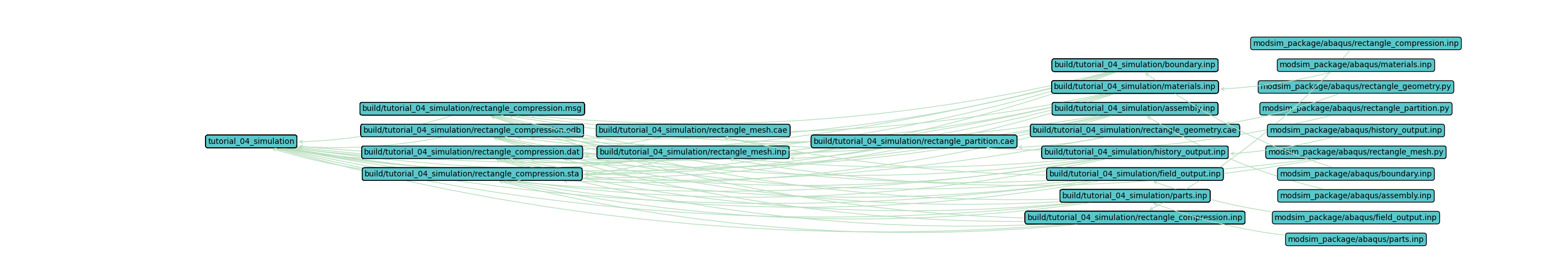
Workflow Visualization#
View the workflow directed graph by running the following command and opening the image in your preferred image viewer.
$ pwd
/home/roppenheimer/waves-tutorials
$ waves visualize tutorial_04_simulation --output-file tutorial_04_simulation.png --width=28 --height=5 --exclude-list /usr/bin .stdout .jnl .prt .com
PS > Get-Location

Path
----
C:\Users\roppenheimer\waves-tutorials

PS > waves visualize tutorial_04_simulation --output-file tutorial_04_simulation.png --width=28 --height=5 --exclude-list .stdout .jnl .prt .com
The output should look similar to the figure below.