Tutorial 08: Data Extraction

Many post-processing activities require a non-proprietary serialization format to provide common access to a mix of analysis libraries and tools. The Parameter Generators of this project uses the xarray dataset and H5 files, so it will be convenient to extract data results to a similar H5 file using matching coordinates for the N-dimensional data.

Abaqus provides a scripting interface and a proprietary, binary output database file containing the simulation results. While this object and interface is good for scripting with the Abaqus kernel and CAE features, the Python interface is limited to the Python 2.7 environment that is shipped with Abaqus. When post-processing requires more Python libraries or other third party tools, it is common to extract a portion of the Abaqus results to an intermediate file. To reduce duplicated effort in extracting Abaqus ODB files to a common format, the ODB Extract command-line utility and the associated waves.scons_extensions.abaqus_extract() builder are provided to parse the output of abaqus odbreport into several xarray dataset objects in an H5 file.

Future releases of WAVES may include extract utilities for other numeric solvers.

References

• WAVES SCons Extensions API: waves.scons_extensions.abaqus_extract()

• SCons Attaching a Builder to a Construction Environment [32]

• ODB Extract CLI

• Xarray [41]

• h5py [43]

• The HDF5 Group command-line-tools [44]

Environment

SCons and WAVES can be installed in a Conda environment with the Conda package manager. See the Conda installation and Conda environment management documentation for more details about using Conda.

Note

The SALib and numpy versions may not need to be this strict for most tutorials. However, Tutorial: Sensitivity Study uncovered some undocumented SALib version sensitivity to numpy surrounding the numpy v2 rollout.

1. Create the tutorials environment if it doesn’t exist

   $ conda create --name waves-tutorial-env --channel conda-forge waves 'scons>=4.6' matplotlib pandas pyyaml xarray seaborn 'numpy>=2' 'salib>=1.5.1' pytest
   

2. Activate the environment

   $ conda activate waves-tutorial-env
   

Some tutorials require additional third-party software that is not available for the Conda package manager. This software must be installed separately and either made available to SConstruct by modifying your system’s PATH or by modifying the SConstruct search paths provided to the waves.scons_extensions.add_program() method.

Warning

STOP! Before continuing, check that the documentation version matches your installed package version.

1. You can find the documentation version in the upper-left corner of the webpage.

2. You can find the installed WAVES version with waves --version.

If they don’t match, you can launch identically matched documentation with the WAVES Command-Line Utility docs subcommand as waves docs.

Directory Structure

3. Create and change to a new project root directory to house the tutorial files if you have not already done so. For example

$ mkdir -p ~/waves-tutorials
$ cd ~/waves-tutorials
$ pwd
/home/roppenheimer/waves-tutorials

Note

If you skipped any of the previous tutorials, run the following commands to create a copy of the necessary tutorial files.

$ pwd
/home/roppenheimer/waves-tutorials
$ waves fetch --overwrite --tutorial 7 && mv tutorial_07_cartesian_product_SConstruct SConstruct
WAVES fetch
Destination directory: '/home/roppenheimer/waves-tutorials'

4. Download and copy the tutorial_07_cartesian_product file to a new file named tutorial_08_data_extraction with the WAVES Command-Line Utility fetch subcommand.

$ pwd
/home/roppenheimer/waves-tutorials
$ waves fetch --overwrite tutorials/tutorial_07_cartesian_product && cp tutorial_07_cartesian_product tutorial_08_data_extraction
WAVES fetch
Destination directory: '/home/roppenheimer/waves-tutorials'

SConscript

A diff against the tutorial_07_cartesian_product file from Tutorial 07: Cartesian Product is included below to help identify the changes made in this tutorial.

waves-tutorials/tutorial_08_data_extraction

--- /home/runner/work/waves/waves/build/docs/tutorials_tutorial_07_cartesian_product
+++ /home/runner/work/waves/waves/build/docs/tutorials_tutorial_08_data_extraction
@@ -149,6 +149,15 @@
         )
     )
 
+    # Extract Abaqus
+    extract_source_list = [set_name / "rectangle_compression.odb"]
+    workflow.extend(
+        env.AbaqusExtract(
+            target=[set_name / "rectangle_compression.h5"],
+            source=extract_source_list,
+        )
+    )
+
 # Comment used in tutorial code snippets: marker-6
 
 # Collector alias based on parent directory name

The only new code in this tutorial adds the waves.scons_extensions.abaqus_extract() builder task. Note that this task falls within the parameterization loop and will be executed once per parameter set. ODB Extract will output two files: rectangle_compression_datasets.h5, which contains h5py paths to the Xarray datasets, and rectangle_compression.h5, which contains h5py native datasets for anything that ODB Extract doesn’t organize into Xarray datasets and a list of group paths pointing at Xarray datasets in rectangle_compression_datasets.h5. The second file also contains external links to the datasets file, so h5py can be used to access all group paths if necessary. Tutorial 09: Post-Processing will introduce an example for accessing and organizing the results files and concatenating the parameter study information.

SConstruct

5. Update the SConstruct file with the changes below.

   • Attach the waves.scons_extensions.abaqus_extract() builder to the construction environment as AbaqusExtract by appending the BUILDERS dictionary.

   • Add tutorial_08_data_extraction to the workflow_configurations list.

A diff against the SConstruct file from Tutorial 07: Cartesian Product is included below to help identify the changes made in this tutorial.

waves-tutorials/SConstruct

--- /home/runner/work/waves/waves/build/docs/tutorials_tutorial_07_cartesian_product_SConstruct
+++ /home/runner/work/waves/waves/build/docs/tutorials_tutorial_08_data_extraction_SConstruct
@@ -92,7 +92,11 @@
 # Comments used in tutorial code snippets: marker-5
 
 # Add builders and pseudo-builders
-env.Append(BUILDERS={})
+env.Append(
+    BUILDERS={
+        "AbaqusExtract": waves.scons_extensions.abaqus_extract(program=env["ABAQUS_PROGRAM"]),
+    }
+)
 
 # Comments used in tutorial code snippets: marker-6
 
@@ -105,6 +109,7 @@
     "tutorial_05_parameter_substitution",
     "tutorial_06_include_files",
     "tutorial_07_cartesian_product",
+    "tutorial_08_data_extraction",
 ]
 for workflow in workflow_configurations:
     build_dir = env["variant_dir_base"] / workflow

Build Targets

6. Build the new targets

$ pwd
/home/roppenheimer/waves-tutorials
$ scons tutorial_08_data_extraction --jobs=4
<output truncated>

Output Files

7. View the output files. The output files should match those introduced in Tutorial 07: Cartesian Product, with the addition of the ODB Extract output files.

$ pwd
/home/roppenheimer/waves-tutorials
$ find build/tutorial_08_data_extraction/ -name "*.h5"
build/tutorial_08_data_extraction/parameter_set2/rectangle_compression.h5
build/tutorial_08_data_extraction/parameter_set2/rectangle_compression_datasets.h5
build/tutorial_08_data_extraction/parameter_set1/rectangle_compression.h5
build/tutorial_08_data_extraction/parameter_set1/rectangle_compression_datasets.h5
build/tutorial_08_data_extraction/parameter_set3/rectangle_compression.h5
build/tutorial_08_data_extraction/parameter_set3/rectangle_compression_datasets.h5
build/tutorial_08_data_extraction/parameter_set0/rectangle_compression.h5
build/tutorial_08_data_extraction/parameter_set0/rectangle_compression_datasets.h5

See the ODB Extract and waves.scons_extensions.abaqus_extract() documentation for an overview of the H5 file structure. You will notice that there are two H5 files per parameter set. The data is organized into a root file, rectangle_compression.h5, that contains the overall file structure, some unsorted meta data, and a list of H5 group paths containing Xarray datasets. The second file, rectangle_compression_datasets.h5, contains the actual Xarray dataset objects. Tutorial 09: Post-Processing will introduce a post-processing task with the waves.scons_extensions.abaqus_extract() H5 output files.

You can explore the structure of each file with The HDF5 Group command-line-tools below (the grep command excludes the large, unsorted data in the /odb group path).

rectangle_compression.h5

$ h5ls -r build/tutorial_08_data_extraction/parameter_set0/rectangle_compression.h5 | grep -v odb
/                        Group
/RECTANGLE               Group
/RECTANGLE/FieldOutputs  Group
/RECTANGLE/FieldOutputs/ALL_ELEMENTS External Link {/home/roppenheimer/waves-tutorials/build/tutorial_08_data_extraction/parameter_set0/rectangle_compression_datasets.h5//RECTANGLE/FieldOutputs/ALL_ELEMENTS}
/RECTANGLE/FieldOutputs/ALL_NODES External Link {/home/roppenheimer/waves-tutorials/build/tutorial_08_data_extraction/parameter_set0/rectangle_compression_datasets.h5//RECTANGLE/FieldOutputs/ALL_NODES}
/RECTANGLE/HistoryOutputs Group
/RECTANGLE/HistoryOutputs/NODES External Link {/home/roppenheimer/waves-tutorials/build/tutorial_08_data_extraction/parameter_set0/rectangle_compression_datasets.h5//RECTANGLE/HistoryOutputs/NODES}
/RECTANGLE/Mesh          External Link {/home/roppenheimer/waves-tutorials/build/tutorial_08_data_extraction/parameter_set0/rectangle_compression_datasets.h5//RECTANGLE/Mesh}
/xarray                  Group
/xarray/Dataset          Dataset {4}

rectangle_compression_datasets.h5

$ h5ls -r waves/tutorials/build/tutorial_08_data_extraction/parameter_set0/rectangle_compression_datasets.h5
/                        Group
/RECTANGLE               Group
/RECTANGLE/FieldOutputs  Group
/RECTANGLE/FieldOutputs/ALL_ELEMENTS Group
/RECTANGLE/FieldOutputs/ALL_ELEMENTS/E Dataset {1, 5, 1, 4, 4}
/RECTANGLE/FieldOutputs/ALL_ELEMENTS/E\ values Dataset {4}
/RECTANGLE/FieldOutputs/ALL_ELEMENTS/S Dataset {1, 5, 1, 4, 4}
/RECTANGLE/FieldOutputs/ALL_ELEMENTS/S\ values Dataset {4}
/RECTANGLE/FieldOutputs/ALL_ELEMENTS/elements Dataset {1}
/RECTANGLE/FieldOutputs/ALL_ELEMENTS/integration\ point Dataset {4}
/RECTANGLE/FieldOutputs/ALL_ELEMENTS/integrationPoint Dataset {1, 4}
/RECTANGLE/FieldOutputs/ALL_ELEMENTS/step Dataset {1}
/RECTANGLE/FieldOutputs/ALL_ELEMENTS/time Dataset {5}
/RECTANGLE/FieldOutputs/ALL_NODES Group
/RECTANGLE/FieldOutputs/ALL_NODES/U Dataset {1, 5, 4, 2}
/RECTANGLE/FieldOutputs/ALL_NODES/U\ values Dataset {2}
/RECTANGLE/FieldOutputs/ALL_NODES/nodes Dataset {4}
/RECTANGLE/FieldOutputs/ALL_NODES/step Dataset {1}
/RECTANGLE/FieldOutputs/ALL_NODES/time Dataset {5}
/RECTANGLE/HistoryOutputs Group
/RECTANGLE/HistoryOutputs/NODES Group
/RECTANGLE/HistoryOutputs/NODES/U1 Dataset {1, 14}
/RECTANGLE/HistoryOutputs/NODES/U2 Dataset {1, 14}
/RECTANGLE/HistoryOutputs/NODES/node Dataset {1}
/RECTANGLE/HistoryOutputs/NODES/step Dataset {1}
/RECTANGLE/HistoryOutputs/NODES/time Dataset {14}
/RECTANGLE/HistoryOutputs/NODES/type Dataset {1}
/RECTANGLE/Mesh          Group
/RECTANGLE/Mesh/CPS4R    Dataset {1}
/RECTANGLE/Mesh/CPS4R_mesh Dataset {1, 4}
/RECTANGLE/Mesh/CPS4R_node Dataset {4}
/RECTANGLE/Mesh/node     Dataset {4}
/RECTANGLE/Mesh/node_location Dataset {4, 3}
/RECTANGLE/Mesh/section_category Dataset {1}
/RECTANGLE/Mesh/vector   Dataset {3}

Each group path directly above a Dataset path entry can be opened with Xarray, e.g. /RECTANGLE/FieldOutputs/ALL_ELEMENTS as

import xarray
extracted_file = "build/tutorial_08_data_extraction/parameter_set0/rectangle_compression.h5"
group_path = "/RECTANGLE/FieldOutputs/ALL_ELEMENTS"
field_outputs = xarray.open_dataset(extracted_file, group=group_path)

The structure is separated into two files to aid automated exploration of the data structure. The root file, rectangle_compression.h5 may be opened with h5py to obtain the Xarray datasets list in the /xarray/Dataset group path. Then the datasets file, rectangle_compression_datasets.h5, may be opened separately with Xarray in the same Python script. This is required because h5py and Xarray can not access the same file at the same time.

In practice when you know the Xarray dataset path(s) relevant to your workflow, you may also go directly to the datasets file.

import xarray
extracted_file = "build/tutorial_08_data_extraction/parameter_set0/rectangle_compression_datasets.h5"
group_path = "/RECTANGLE/FieldOutputs/ALL_ELEMENTS"
field_outputs = xarray.open_dataset(extracted_file, group=group_path)

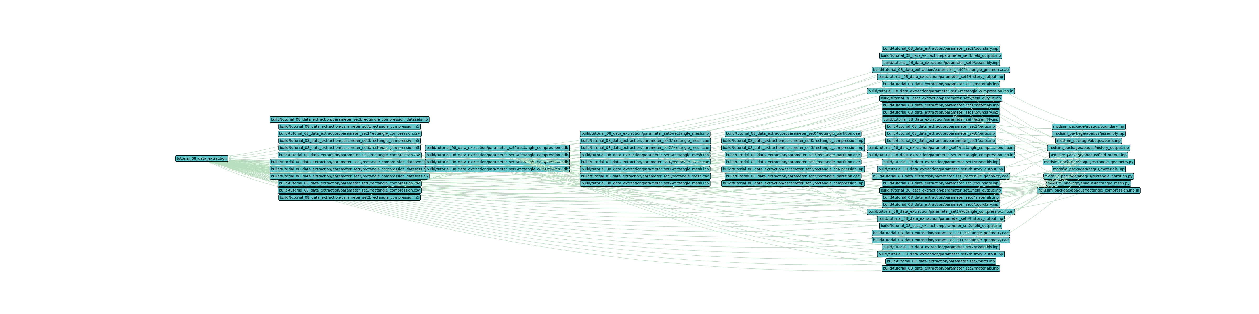
Workflow Visualization

View the workflow directed graph by running the following command and opening the image in your preferred image viewer. First, plot the workflow with all parameter sets.

$ pwd
/home/roppenheimer/waves-tutorials
$ waves visualize tutorial_08_data_extraction --output-file tutorial_08_data_extraction.png --width=48 --height=12 --exclude-list /usr/bin .stdout .jnl .prt .com .msg .dat .sta

The output should look similar to the figure below.

Now plot the workflow with only the first set, set0.

$ pwd
/home/roppenheimer/waves-tutorials
$ waves visualize tutorial_08_data_extraction --output-file tutorial_08_data_extraction_set0.png --width=46 --height=6 --exclude-list /usr/bin .stdout .jnl .prt .com .msg .dat .sta --exclude-regex "set[1-9]"

The output should look similar to the figure below.

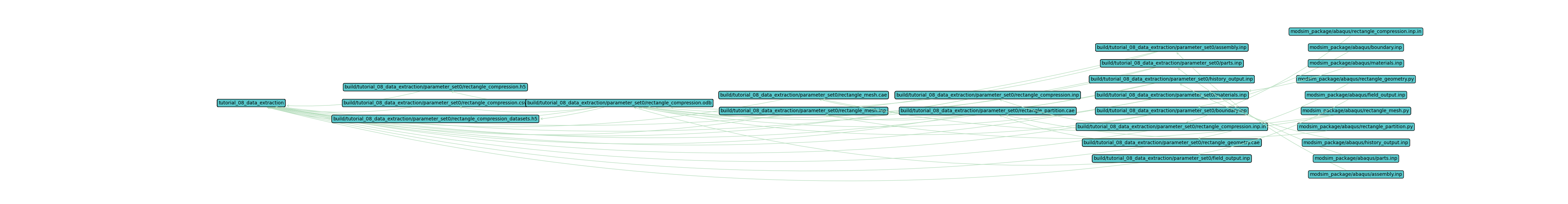
This single set directed graph image should look very similar to the Tutorial 07: Cartesian Product directed graph. The data extraction step has added the *.h5 files which take the proprietary *.odb data format and provide h5py and xarray dataset files.