Tutorial 09: Post-Processing#
References#
WAVES SCons Extensions API:
waves.scons_extensions.python_builder_factory()WAVES Parameter Generators API:
waves.parameter_generators.CartesianProduct()Xarray and the xarray dataset [46, 47]
matplotlib [51]
Environment#
SCons and WAVES can be installed in a Conda environment with the Conda package manager. See the Conda installation and Conda environment management documentation for more details about using Conda.
Note
The SALib and numpy versions may not need to be this strict for most tutorials. However, Tutorial: Sensitivity Study uncovered some undocumented SALib version sensitivity to numpy surrounding the numpy v2 rollout.
Create the tutorials environment if it doesn’t exist
$ conda create --name waves-tutorial-env --channel conda-forge waves 'scons>=4.6' matplotlib pandas pyyaml xarray seaborn 'numpy>=2' 'salib>=1.5.1' pytest
PS > conda create --name waves-tutorial-env --channel conda-forge waves scons matplotlib pandas pyyaml xarray seaborn numpy salib pytest
Activate the environment
$ conda activate waves-tutorial-env
PS > conda activate waves-tutorial-env
Some tutorials require additional third-party software that is not available for the Conda package manager. This
software must be installed separately and either made available to SConstruct by modifying your system’s PATH or by
modifying the SConstruct search paths provided to the waves.scons_extensions.add_program() method.
Warning
STOP! Before continuing, check that the documentation version matches your installed package version.
You can find the documentation version in the upper-left corner of the webpage.
You can find the installed WAVES version with
waves --version.
If they don’t match, you can launch identically matched documentation with the WAVES Command-Line Utility
docs subcommand as waves docs.
Directory Structure#
Create and change to a new project root directory to house the tutorial files if you have not already done so. For example
$ mkdir -p ~/waves-tutorials
$ cd ~/waves-tutorials
$ pwd
/home/roppenheimer/waves-tutorials
PS > New-Item $HOME\waves-tutorials -ItemType "Directory"
PS > Set-Location $HOME\waves-tutorials
PS > Get-Location

Path
----
C:\Users\roppenheimer\waves-tutorials
Note
If you skipped any of the previous tutorials, run the following commands to create a copy of the necessary tutorial files.
$ pwd
/home/roppenheimer/waves-tutorials
$ waves fetch --overwrite --tutorial 8 && mv tutorial_08_data_extraction_SConstruct SConstruct
WAVES fetch
Destination directory: '/home/roppenheimer/waves-tutorials'
PS > Get-Location

Path
----
C:\Users\roppenheimer\waves-tutorials

PS > waves fetch --overwrite --tutorial 8 && Move-Item tutorial_08_data_extraction_SConstruct SConstruct -Force
WAVES fetch
Destination directory: 'C:\Users\roppenheimer\waves-tutorials'
Download and copy the
tutorial_08_data_extraction.sconsfile to a new file namedtutorial_09_post_processing.sconswith the WAVES Command-Line Utility fetch subcommand.
$ pwd
/home/roppenheimer/waves-tutorials
$ waves fetch --overwrite tutorials/tutorial_08_data_extraction.scons && cp tutorial_08_data_extraction.scons tutorial_09_post_processing.scons
WAVES fetch
Destination directory: '/home/roppenheimer/waves-tutorials'
PS > Get-Location

Path
----
C:\Users\roppenheimer\waves-tutorials

PS > waves fetch --overwrite tutorials\tutorial_08_data_extraction.scons && Copy-Item tutorial_08_data_extraction.scons tutorial_09_post_processing.scons
WAVES fetch
Destination directory: 'C:\Users\roppenheimer\waves-tutorials'
SConscript#
A diff against the tutorial_08_data_extraction.scons file from Tutorial 08: Data Extraction is included below to help identify the
changes made in this tutorial.
waves-tutorials/tutorial_09_post_processing.scons
--- /home/runner/work/waves/waves/build/docs/tutorials_tutorial_08_data_extraction.scons
+++ /home/runner/work/waves/waves/build/docs/tutorials_tutorial_09_post_processing.scons
@@ -160,6 +160,22 @@

 # Comment used in tutorial code snippets: marker-6

+# Post-processing
+post_processing_source = [
+    pathlib.Path(set_name) / "rectangle_compression_datasets.h5"
+    for set_name in parameter_generator.parameter_study_to_dict()
+]
+script_options = "--input-file ${SOURCES[2:].abspath}"
+script_options += " --output-file ${TARGET.file} --x-units mm/mm --y-units MPa"
+script_options += " --parameter-study-file ${SOURCES[1].abspath}"
+workflow.extend(
+    env.PythonScript(
+        target=["stress_strain_comparison.pdf", "stress_strain_comparison.csv"],
+        source=["#/modsim_package/python/post_processing.py", parameter_study_file.name, *post_processing_source],
+        subcommand_options=script_options,
+    )
+)
+
 # Collector alias based on parent directory name
 env.Alias(workflow_name, workflow)
 env.Alias(f"{workflow_name}_datacheck", datacheck)
The Python 3 post-processing script is executed with the waves.scons_extensions.python_builder_factory() builder
from the waves.scons_extensions.WAVESEnvironment construction environment. This builder behaves similarly to
the waves.scons_extensions.abaqus_journal_builder_factory() builders introduced in earlier tutorials. By default,
the builder uses the same Python interpreter as the launching Conda environment where SCons and WAVES are
installed. So unlike Abaqus Python, the user has full control over the Python execution environment.
Advanced SCons users may be tempted to write an SCons Python function builder for the post-processing task [31]. A Python function builder would have the advantage of allowing users to pass Python objects to the task definition directly. This would eliminate the need to read an intermediate YAML file for the plot selection dictionary, for instance.
Here we use the post_processing.py CLI instead of the module’s API for the task definition because the
post-processing will include plotting with matplotlib [51], which is not thread-safe
[53]. When the CLI is used, multiple post-processing tasks from separate workflows can be
executed in parallel because each task will be launched from a separate Python main process. Care must still be taken to
ensure that the post-processing tasks do not write to the same files, however.
Post-processing script#
In the
waves-tutorials/modsim_package/pythondirectory, create a file calledpost_processing.pyusing the contents below.
Note
Depending on the memory and disk resources available and the size of the simulation workflow results, modsim projects may need to review the Xarray documentation for resource management specific to the projects’ use case.
waves-tutorials/modsim_package/python/post_processing.py
#!/usr/bin/env python
"""Example of catenating WAVES parameter study results and definition."""

import argparse
import pathlib
import sys

import matplotlib.pyplot
import xarray
import yaml
from waves.parameter_generators import SET_COORDINATE_KEY

default_selection_dict = {
    "E values": "E22",
    "S values": "S22",
    "elements": 1,
    "step": "Step-1",
    "integration point": 0,
}


def combine_data(
    input_files: list[str | pathlib.Path],
    group_path: str,
    concat_coord: str,
) -> xarray.Dataset:
    """Combine input data files into one dataset.

    :param input_files: list of path-like or file-like objects pointing to h5netcdf files
        containing Xarray Datasets
    :param group_path: The h5netcdf group path locating the Xarray Dataset in the input files.
    :param concat_coord: Name of dimension

    :returns: Combined data
    """
    paths = [pathlib.Path(input_file).resolve() for input_file in input_files]
    data_generator = (
        xarray.open_dataset(path, group=group_path, engine="h5netcdf").assign_coords({concat_coord: path.parent.name})
        for path in paths
    )
    combined_data = xarray.concat(data_generator, concat_coord, join="outer", compat="no_conflicts")
    combined_data.close()

    return combined_data


def merge_parameter_study(
    parameter_study_file: str | pathlib.Path,
    combined_data: xarray.Dataset,
) -> xarray.Dataset:
    """Merge parameter study to existing dataset.

    :param parameter_study_file: path-like or file-like object containing the parameter study dataset. Assumes the
        h5netcdf file contains only a single dataset at the root group path, .e.g. ``/``.
    :param combined_data: XArray Dataset that will be merged.

    :returns: Combined data
    """
    parameter_study = xarray.open_dataset(parameter_study_file, engine="h5netcdf")
    combined_data = combined_data.merge(parameter_study)
    parameter_study.close()
    return combined_data


def save_plot(
    combined_data: xarray.Dataset,
    x_var: str,
    y_var: str,
    selection_dict: dict,
    concat_coord: str,
    output_file: str | pathlib.Path,
) -> None:
    """Save scatter plot with given x and y labels.

    :param combined_data: XArray Dataset that will be plotted.
    :param x_var: The independent (x-axis) variable key name for the Xarray Dataset "data variable"
    :param y_var: The dependent (y-axis) variable key name for the Xarray Dataset "data variable"
    :param selection_dict: Dictionary to define the down selection of data to be plotted. Dictionary ``key: value``
        pairs must match the data variables and coordinates of the expected Xarray Dataset object.
    :param concat_coord: Name of dimension for which you want multiple lines plotted.
    :param output_file: The plot file name. Relative or absolute path.
    """
    # Plot
    combined_data.sel(selection_dict).plot.scatter(x=x_var, y=y_var, hue=concat_coord)
    matplotlib.pyplot.title(None)
    matplotlib.pyplot.savefig(output_file)


def save_table(
    combined_data: xarray.Dataset,
    selection_dict: dict,
    output_file: str | pathlib.Path,
) -> None:
    """Save csv table.

    :param combined_data: XArray Dataset to be written as a CSV.
    :param selection_dict: Dictionary to define the down selection of data to be plotted. Dictionary ``key: value``
        pairs must match the data variables and coordinates of the expected Xarray Dataset object.
    :param output_file: The CSV file name. Relative or absolute path.
    """
    combined_data.sel(selection_dict).to_dataframe().to_csv(output_file)


def main(
    input_files: list[pathlib.Path],
    output_file: pathlib.Path,
    group_path: str,
    x_var: str,
    x_units: str,
    y_var: str,
    y_units: str,
    selection_dict: dict,
    parameter_study_file: pathlib.Path | None = None,
) -> None:
    """Catenate ``input_files`` datasets along the ``set_name`` dimension and plot selected data.

    Optionally merges the parameter study results datasets with the parameter study definition dataset, where the
    parameter study dataset file is assumed to be written by a WAVES parameter generator.

    :param list input_files: list of path-like or file-like objects pointing to h5netcdf files containing Xarray
        Datasets
    :param str output_file: The plot file name. Relative or absolute path.
    :param str group_path: The h5netcdf group path locating the Xarray Dataset in the input files.
    :param str x_var: The independent (x-axis) variable key name for the Xarray Dataset "data variable"
    :param str x_units: The independent (x-axis) units
    :param str y_var: The dependent (y-axis) variable key name for the Xarray Dataset "data variable"
    :param str y_units: The dependent (y-axis) units
    :param dict selection_dict: Dictionary to define the down selection of data to be plotted. Dictionary ``key: value``
        pairs must match the data variables and coordinates of the expected Xarray Dataset object.
    :param str parameter_study_file: path-like or file-like object containing the parameter study dataset. Assumes the
        h5netcdf file contains only a single dataset at the root group path, .e.g. ``/``.
    """
    output_file = pathlib.Path(output_file)
    output_csv = output_file.with_suffix(".csv")
    concat_coord = SET_COORDINATE_KEY

    # Build single dataset along the "set_name" dimension
    combined_data = combine_data(input_files, group_path, concat_coord)

    # Open and merge WAVES parameter study if provided
    if parameter_study_file:
        combined_data = merge_parameter_study(parameter_study_file, combined_data)

    # Add units
    combined_data[x_var].attrs["units"] = x_units
    combined_data[y_var].attrs["units"] = y_units

    # Tutorial 09: post processing print statement to view data structure
    print(combined_data)

    # Output files
    save_plot(combined_data, x_var, y_var, selection_dict, concat_coord, output_file)
    save_table(combined_data, selection_dict, output_csv)

    # Clean up open files
    combined_data.close()


def get_parser() -> argparse.ArgumentParser:
    """Return parser for CLI options."""
    script_name = pathlib.Path(__file__)
    default_output_file = f"{script_name.stem}.pdf"
    default_group_path = "RECTANGLE/FieldOutputs/ALL_ELEMENTS"
    default_x_var = "E"
    default_y_var = "S"
    default_parameter_study_file = None

    prog = f"python {script_name.name} "
    cli_description = (
        "Read Xarray Datasets and plot stress-strain comparisons as a function of parameter set name. "
        " Save to ``output_file``."
    )
    parser = argparse.ArgumentParser(description=cli_description, prog=prog)
    required_named = parser.add_argument_group("required named arguments")
    required_named.add_argument(
        "-i",
        "--input-file",
        nargs="+",
        type=pathlib.Path,
        required=True,
        help="The Xarray Dataset file(s)",
    )
    required_named.add_argument(
        "--x-units",
        type=str,
        required=True,
        help="The dependent (x-axis) units string.",
    )
    required_named.add_argument(
        "--y-units",
        type=str,
        required=True,
        help="The independent (y-axis) units string.",
    )

    parser.add_argument(
        "-o",
        "--output-file",
        type=pathlib.Path,
        default=default_output_file,
        help=(
            "The output file for the stress-strain comparison plot with extension, "
            "e.g. ``output_file.pdf``. Extension must be supported by matplotlib. File stem is also "
            "used for the CSV table output, e.g. ``output_file.csv``. (default: %(default)s)"
        ),
    )
    parser.add_argument(
        "-g",
        "--group-path",
        type=str,
        default=default_group_path,
        help="The h5py group path to the dataset object (default: %(default)s)",
    )
    parser.add_argument(
        "-x",
        "--x-var",
        type=str,
        default=default_x_var,
        help="The independent (x-axis) variable name (default: %(default)s)",
    )
    parser.add_argument(
        "-y",
        "--y-var",
        type=str,
        default=default_y_var,
        help="The dependent (y-axis) variable name (default: %(default)s)",
    )
    parser.add_argument(
        "-s",
        "--selection-dict",
        type=pathlib.Path,
        default=None,
        help=(
            "The YAML formatted dictionary file to define the down selection of data to be plotted. "
            "Dictionary key: value pairs must match the data variables and coordinates of the "
            "expected Xarray Dataset object. If no file is provided, the a default selection dict "
            f"will be used (default: {default_selection_dict})"
        ),
    )
    parser.add_argument(
        "-p",
        "--parameter-study-file",
        type=pathlib.Path,
        default=default_parameter_study_file,
        help="An optional h5 file with a WAVES parameter study Xarray Dataset (default: %(default)s)",
    )

    return parser


if __name__ == "__main__":
    parser = get_parser()
    args = parser.parse_args()
    if not args.selection_dict:
        selection_dict = default_selection_dict
    else:
        with args.selection_dict.open(mode="r") as input_yaml:
            selection_dict = yaml.safe_load(input_yaml)
    sys.exit(
        main(
            input_files=args.input_file,
            output_file=args.output_file,
            group_path=args.group_path,
            x_var=args.x_var,
            x_units=args.x_units,
            y_var=args.y_var,
            y_units=args.y_units,
            selection_dict=selection_dict,
            parameter_study_file=args.parameter_study_file,
        )
    )
The post-processing script is the first Python 3 script introduced in the core tutorials. It differs from the Abaqus journal files by executing against the Python 3 interpreter of the launching Conda environment where WAVES is installed. Unlike the Abaqus Python 2 environment used to execute journal files, users have direct control over this environment and can use the full range of Python packages available with the Conda package manager.
Additionally, the full Python 3 environment allows greater flexibility in unit testing. The post-processing script has been broken into small units of work for ease of testing, which will be introduced in Tutorial 10: Unit Testing. Testing is important to verify that data manipulation is performed correctly. As an added benefit, writing small, single-purpose functions makes project code more re-usable and the project can build a small library of common utilities.
While it is possible to unit test Abaqus Python 2 scripts, most operations in the tutorial journal files require operations on real geometry files, which requires system tests. Tutorial 11: Regression Testing will introduce an example solution to performing system tests on simulation workflows.
Take some time to review the individual functions and their documentation, both in the source file and as rendered by
the documentation. Most of the behavior is explained in the References third-party
package documentation or the Python documentation. Most of the Python built-in operations should look familiar, but
novice Python users may be unfamiliar with the generator expression stored in the data_generator variable of the
combine_data function. Python generator expressions behave similarly to list comprehensions. A generator
expression is used here to avoid performing file I/O operations until the post-processing script is ready to catenate
the results files into a single xarray dataset.
The script API and CLI are included in the WAVES-TUTORIAL API: post_processing.py and WAVES-TUTORIAL CLI: post_processing.py, respectively. Generally, this example script tries to model the separation of: data input, data processing, data output, and status reporting. The Software Carpentry: Python Novice is a good introduction to Python programming practices [8].
SConstruct#
A diff against the SConstruct file from Tutorial 08: Data Extraction is included below to help identify the
changes made in this tutorial.
waves-tutorials/SConstruct
--- /home/runner/work/waves/waves/build/docs/tutorials_tutorial_08_data_extraction_SConstruct
+++ /home/runner/work/waves/waves/build/docs/tutorials_tutorial_09_post_processing_SConstruct
@@ -1,5 +1,5 @@
 #! /usr/bin/env python
-"""Configure the WAVES data extraction tutorial."""
+"""Configure the WAVES post-processing tutorial."""

 import os
 import pathlib
@@ -111,6 +111,7 @@
     "tutorial_06_include_files.scons",
     "tutorial_07_cartesian_product.scons",
     "tutorial_08_data_extraction.scons",
+    "tutorial_09_post_processing.scons",
 ]
 for workflow in workflow_configurations:
     build_dir = env["variant_dir_base"] / pathlib.Path(workflow).stem
Build Targets#
Build the new targets
$ pwd
/home/roppenheimer/waves-tutorials
$ scons tutorial_09_post_processing --jobs=4
<output truncated>
PS > Get-Location

Path
----
C:\Users\roppenheimer\waves-tutorials

PS > scons tutorial_09_post_processing --jobs=4
<output truncated>
Output Files#
Observe the catenated parameter results and paramter study dataset in the post-processing task’s STDOUT file
$ tree build/tutorial_09_post_processing/ -L 1
build/tutorial_09_post_processing/
|-- parameter_set0
|-- parameter_set1
|-- parameter_set2
|-- parameter_set3
|-- parameter_study.h5
|-- stress_strain_comparison.csv
|-- stress_strain_comparison.pdf
`-- stress_strain_comparison.pdf.stdout

4 directories, 4 files
$ cat build/tutorial_09_post_processing/stress_strain_comparison.pdf.stdout
<xarray.Dataset>
Dimensions:             (step: 1, time: 5, elements: 1, integration point: 4,
                         E values: 4, set_name: 4, S values: 4)
Coordinates:
  * step                (step) object 'Step-1'
  * time                (time) float64 0.0175 0.07094 0.2513 0.86 1.0
  * elements            (elements) int64 1
    integrationPoint    (elements, integration point) float64 1.0 nan nan nan
  * E values            (E values) object 'E11' 'E22' 'E33' 'E12'
  * S values            (S values) object 'S11' 'S22' 'S33' 'S12'
  * set_name            (set_name) <U14 'parameter_set0' ... 'parameter...
    set_hash            (set_name) object ...
Dimensions without coordinates: integration point
Data variables:
    E                   (set_name, step, time, elements, integration point, E values) float32 ...
    S                   (set_name, step, time, elements, integration point, S values) float32 ...
    displacement        (set_name) float64 ...
    global_seed         (set_name) float64 ...
    height              (set_name) float64 ...
    width               (set_name) float64 ...
PS > Get-ChildItem build\tutorial_09_post_processing\

    Directory: C:\Users\roppenheimer\waves-tutorials\build\tutorial_09_post_processing

Mode                 LastWriteTime         Length Name
----                 -------------         ------ ----
d----            6/9/2023  4:32 PM                parameter_set0
d----            6/9/2023  4:32 PM                parameter_set1
d----            6/9/2023  4:32 PM                parameter_set2
d----            6/9/2023  4:32 PM                parameter_set3
-a---            6/9/2023  4:32 PM           9942 parameter_study.h5
-a---            6/9/2023  4:32 PM           2609 stress_strain_comparison.csv
-a---            6/9/2023  4:32 PM          12061 stress_strain_comparison.pdf
-a---            6/9/2023  4:32 PM           1160 stress_strain_comparison.pdf.stdout

PS > Get-Content build\tutorial_09_post_processing\stress_strain_comparison.pdf.stdout
<xarray.Dataset> Size: 4kB
Dimensions:           (set_name: 4, step: 1, time: 5, elements: 1,
                       integration point: 4, E values: 4, S values: 4)
Coordinates:
  * E values          (E values) <U3 48B 'E11' 'E22' 'E33' 'E12'
  * S values          (S values) <U3 48B 'S11' 'S22' 'S33' 'S12'
  * elements          (elements) int64 8B 1
    integrationPoint  (elements, integration point) float64 32B 1.0 nan nan nan
  * step              (step) <U6 24B 'Step-1'
  * time              (time) float64 40B 0.0175 0.07094 0.2513 0.86 1.0
  * set_name          (set_name) <U14 224B 'parameter_set0' ... 'parameter_set3'
    set_hash          (set_name) <U32 512B ...
Dimensions without coordinates: integration point
Data variables:
    E                 (set_name, step, time, elements, integration point, E values) float32 1kB ...
    S                 (set_name, step, time, elements, integration point, S values) float32 1kB ...
    width             (set_name) float64 32B ...
    height            (set_name) float64 32B ...
    global_seed       (set_name) float64 32B ...
    displacement      (set_name) float64 32B ...
The purpose of catenating the parameter set simulations with the parameter study definition is to examine the connections between output quantities of interest as a function of the parameter study inputs. Working from a single Xarray dataset makes sensitivity studies easier to conduct. In this tutorial, a qualitative comparison is provided in the stress-strain comparison plot, where each parameter set is plotted as a separate series and identified in the legend.
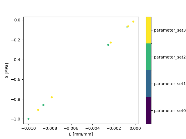
Note that in this example, most of the parameter sets are expected to overlap with differences as a function of the geometric parameters. Review the parameter study introduced in Tutorial 07: Cartesian Product and the contents of the parameter_study.h5 file to identify the expected differences in the stress-strain response.
The ModSim Templates provided by WAVES contain a similar parameter study for mesh convergence as a template for new projects. The fetch subcommand may be used to recursively fetch directories or to fetch individual files from both the ModSim Templates and the tutorials.
Workflow Visualization#
View the workflow directed graph by running the following command and opening the image in your preferred image viewer.
Plot the workflow with only the first set, set0.
$ pwd
/home/roppenheimer/waves-tutorials
$ waves visualize tutorial_09_post_processing --output-file tutorial_09_post_processing_set0.png --width=54 --height=8 --exclude-list /usr/bin .stdout .jnl .prt .com .msg .dat .sta --exclude-regex "set[1-9]"
PS > Get-Location

Path
----
C:\Users\roppenheimer\waves-tutorials

PS > waves visualize tutorial_09_post_processing --output-file tutorial_09_post_processing_set0.png --width=54 --height=8 --exclude-list .stdout .jnl .prt .com .msg .dat .sta --exclude-regex "set[1-9]"
The output should look similar to the figure below.
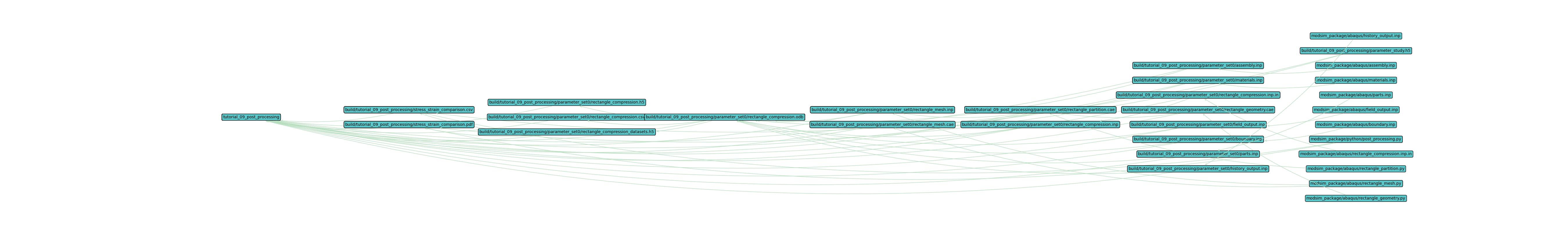
As in Tutorial 08: Data Extraction, the directed graph has not changed much. This tutorial adds the *.pdf plot
of stress vs. strain.