Tutorial 07: Cartesian Product#
References#
WAVES Parameter Generators API:
waves.parameter_generators.CartesianProduct()Xarray and the xarray dataset [46, 47]
Environment#
SCons and WAVES can be installed in a Conda environment with the Conda package manager. See the Conda installation and Conda environment management documentation for more details about using Conda.
Note
The SALib and numpy versions may not need to be this strict for most tutorials. However, Tutorial: Sensitivity Study uncovered some undocumented SALib version sensitivity to numpy surrounding the numpy v2 rollout.
Create the tutorials environment if it doesn’t exist
$ conda create --name waves-tutorial-env --channel conda-forge waves 'scons>=4.6' matplotlib pandas pyyaml xarray seaborn 'numpy>=2' 'salib>=1.5.1' pytest
PS > conda create --name waves-tutorial-env --channel conda-forge waves scons matplotlib pandas pyyaml xarray seaborn numpy salib pytest
Activate the environment
$ conda activate waves-tutorial-env
PS > conda activate waves-tutorial-env
Some tutorials require additional third-party software that is not available for the Conda package manager. This
software must be installed separately and either made available to SConstruct by modifying your system’s PATH or by
modifying the SConstruct search paths provided to the waves.scons_extensions.add_program() method.
Warning
STOP! Before continuing, check that the documentation version matches your installed package version.
You can find the documentation version in the upper-left corner of the webpage.
You can find the installed WAVES version with
waves --version.
If they don’t match, you can launch identically matched documentation with the WAVES Command-Line Utility
docs subcommand as waves docs.
Directory Structure#
Create and change to a new project root directory to house the tutorial files if you have not already done so. For example
$ mkdir -p ~/waves-tutorials
$ cd ~/waves-tutorials
$ pwd
/home/roppenheimer/waves-tutorials
PS > New-Item $HOME\waves-tutorials -ItemType "Directory"
PS > Set-Location $HOME\waves-tutorials
PS > Get-Location

Path
----
C:\Users\roppenheimer\waves-tutorials
Note
If you skipped any of the previous tutorials, run the following commands to create a copy of the necessary tutorial files.
$ pwd
/home/roppenheimer/waves-tutorials
$ waves fetch --overwrite --tutorial 6 && mv tutorial_06_include_files_SConstruct SConstruct
WAVES fetch
Destination directory: '/home/roppenheimer/waves-tutorials'
PS > Get-Location

Path
----
C:\Users\roppenheimer\waves-tutorials

PS > waves fetch --overwrite --tutorial 6 && Move-Item tutorial_06_include_files_SConstruct SConstruct -Force
WAVES fetch
Destination directory: 'C:\Users\roppenheimer\waves-tutorials'
Download and copy the
tutorial_06_include_files.sconsfile to a new file namedtutorial_07_cartesian_product.sconswith the WAVES Command-Line Utility fetch subcommand.
$ pwd
/home/roppenheimer/waves-tutorials
$ waves fetch --overwrite tutorials/tutorial_06_include_files.scons && cp tutorial_06_include_files.scons tutorial_07_cartesian_product.scons
WAVES fetch
Destination directory: '/home/roppenheimer/waves-tutorials'
PS > Get-Location

Path
----
C:\Users\roppenheimer\waves-tutorials

PS > waves fetch --overwrite tutorials\tutorial_06_include_files.scons && Copy-Item tutorial_06_include_files.scons tutorial_07_cartesian_product.scons
WAVES fetch
Destination directory: 'C:\Users\roppenheimer\waves-tutorials'
Parameter Study File#
In this tutorial, we will use an included parameter study python file to define a parameter study using a Cartesian Product sampling methodology.
What is Cartesian Product
A “cartesian product” is a set of all ordered pairs of the elements for a series of list objects. Another commonly used synonym for Cartesian Product is Full Factorial.
Take a parameter study defined by variables A which has three samples, B which has two samples, and C
which has one sample. The result will be a parameter study that contains six (3x2x1) simulations.
For more information, see this Cartesian Product Wiki page.
Create a new file
modsim_package/python/rectangle_compression_cartesian_product.pyfrom the content below.
waves-tutorials/modsim_package/python/rectangle_compression_cartesian_product.py
"""Parameter sets and schemas for the rectangle compression simulation."""


def parameter_schema(
    width: list[float] | tuple[float, ...] = (1.0, 1.1),
    height: list[float] | tuple[float, ...] = (1.0, 1.1),
    global_seed: list[float] | tuple[float, ...] = (1.0,),
    displacement: list[float] | tuple[float, ...] = (-0.01,),
) -> dict[str, list[float]]:
    """Return WAVES CartesianProduct parameter schema.

    :param width: The rectangle width
    :param height: The rectangle height
    :param global_seed: The global mesh seed size
    :param displacement: The rectangle top surface displacement

    :returns: WAVES CartesianProduct parameter schema
    """
    schema = {
        "width": list(width),
        "height": list(height),
        "global_seed": list(global_seed),
        "displacement": list(displacement),
    }
    return schema
The rectangle_compression_cartesian_product.py file you just created is very similar to the
rectangle_compression_nominal.py file from Tutorial 06: Include Files. The significant difference between
the two files is the new definition of multiple values for the width and height parameters. Also note that the
global_seed and displacement parameters are both defined with a list, even though the parameters only have a
single value. The waves.parameter_generators.CartesianProduct() API explains this requirement for the “schema
values” to be an iterable. You can view the parameter schema documentation in the WAVES-TUTORIAL API for
rectangle_compression_cartesian_product.py.
In the parameter_schema, we have defined two parameters with two samples each and two parameters with one sample
each. This will result in four (2x2x1x1) total simulations.
SConscript#
The diff for changes in the SConscript file for this tutorial is extensive because of the for loop indent
wrapping the task generation for each parameter set. For convenience, the full source file is included below to aid in a
wholesale copy and paste when creating the new SConscript file.
Note
In the Directory Structure section of this tutorial, you were instructed to
copy the tutorial_06_include_files.scons file to the tutorial_07_cartesian_product.scons file. If you prefer, you may
start with a blank tutorial_07_cartesian_product.scons file and simply copy and paste the contents below into your
blank file.
After viewing the full file contents below, continue to read the
Step-By-Step SConscript Discussion for building the
tutorial_07_cartesian_product.scons file from scratch.
waves-tutorials/tutorial_07_cartesian_product.scons
#! /usr/bin/env python
"""Rectangle compression workflow.

Requires the following ``SConscript(..., exports={})``

* ``env`` - The SCons construction environment with the following required keys

  * ``unconditional_build`` - Boolean flag to force building of conditionally ignored targets
  * ``abaqus`` - String path for the Abaqus executable
"""

import pathlib

import waves

from modsim_package.python.rectangle_compression_cartesian_product import parameter_schema

# Inherit the parent construction environment
Import("env")

# Comment used in tutorial code snippets: marker-1

# Simulation variables
build_directory = pathlib.Path(Dir(".").abspath)
workflow_name = build_directory.name
parameter_study_file = build_directory / "parameter_study.h5"

# Collect the target nodes to build a concise alias for all targets
workflow = []
datacheck = []

# Comment used in tutorial code snippets: marker-2

# Parameter Study with Cartesian Product
parameter_generator = waves.parameter_generators.CartesianProduct(
    parameter_schema(),
    output_file=parameter_study_file,
    previous_parameter_study=parameter_study_file,
)
parameter_generator.write()

# Comment used in tutorial code snippets: marker-3

# Parameterized targets must live inside current simulation_variables for loop
for set_name, parameters in parameter_generator.parameter_study_to_dict().items():
    set_path = pathlib.Path(set_name)
    simulation_variables = parameters

    # Comment used in tutorial code snippets: marker-4

    # Geometry
    workflow.extend(
        env.AbaqusJournal(
            target=[set_path / "rectangle_geometry.cae", set_path / "rectangle_geometry.jnl"],
            source=["#/modsim_package/abaqus/rectangle_geometry.py"],
            subcommand_options="--width ${width} --height ${height}",
            **simulation_variables,
        )
    )

    # Partition
    workflow.extend(
        env.AbaqusJournal(
            target=[set_path / "rectangle_partition.cae", set_path / "rectangle_partition.jnl"],
            source=["#/modsim_package/abaqus/rectangle_partition.py", set_path / "rectangle_geometry.cae"],
            subcommand_options="--width ${width} --height ${height}",
            **simulation_variables,
        )
    )

    # Mesh
    workflow.extend(
        env.AbaqusJournal(
            target=[
                set_path / "rectangle_mesh.inp",
                set_path / "rectangle_mesh.cae",
                set_path / "rectangle_mesh.jnl",
            ],
            source=["#/modsim_package/abaqus/rectangle_mesh.py", set_path / "rectangle_partition.cae"],
            subcommand_options="--global-seed ${global_seed}",
            **simulation_variables,
        )
    )

    # SolverPrep
    copy_source_list = [
        "#/modsim_package/abaqus/rectangle_compression.inp.in",
        "#/modsim_package/abaqus/assembly.inp",
        "#/modsim_package/abaqus/boundary.inp",
        "#/modsim_package/abaqus/field_output.inp",
        "#/modsim_package/abaqus/materials.inp",
        "#/modsim_package/abaqus/parts.inp",
        "#/modsim_package/abaqus/history_output.inp",
    ]
    workflow.extend(
        env.CopySubstfile(
            copy_source_list,
            substitution_dictionary=env.SubstitutionSyntax(simulation_variables),
            build_subdirectory=set_path,
        )
    )

    # Comment used in tutorial code snippets: marker-5

    # Abaqus Solve
    solve_source_list = [
        set_path / "rectangle_compression.inp",
        set_path / "assembly.inp",
        set_path / "boundary.inp",
        set_path / "field_output.inp",
        set_path / "materials.inp",
        set_path / "parts.inp",
        set_path / "history_output.inp",
        set_path / "rectangle_mesh.inp",
    ]

    datacheck.extend(
        env.AbaqusSolver(
            target=[
                set_path / "rectangle_compression_DATACHECK.odb",
                set_path / "rectangle_compression_DATACHECK.dat",
                set_path / "rectangle_compression_DATACHECK.msg",
                set_path / "rectangle_compression_DATACHECK.com",
                set_path / "rectangle_compression_DATACHECK.prt",
                set_path / "rectangle_compression_DATACHECK.023",
                set_path / "rectangle_compression_DATACHECK.mdl",
                set_path / "rectangle_compression_DATACHECK.sim",
                set_path / "rectangle_compression_DATACHECK.stt",
            ],
            source=solve_source_list,
            job="rectangle_compression_DATACHECK",
            program_options="-double both -datacheck",
        )
    )

    workflow.extend(
        env.AbaqusSolver(
            target=[
                set_path / "rectangle_compression.odb",
                set_path / "rectangle_compression.dat",
                set_path / "rectangle_compression.msg",
                set_path / "rectangle_compression.com",
                set_path / "rectangle_compression.prt",
                set_path / "rectangle_compression.sta",
            ],
            source=solve_source_list,
            job="rectangle_compression",
            program_options="-double both",
        )
    )

# Comment used in tutorial code snippets: marker-6

# Collector alias based on parent directory name
env.Alias(workflow_name, workflow)
env.Alias(f"{workflow_name}_datacheck", datacheck)

if not env["unconditional_build"] and not env["ABAQUS_PROGRAM"]:
    print(f"Program 'abaqus' was not found in construction environment. Ignoring '{workflow_name}' target(s)")
    Ignore([".", workflow_name], workflow)
    Ignore([".", f"{workflow_name}_datacheck"], datacheck)
Step-By-Step SConscript Discussion#
waves-tutorials/tutorial_07_cartesian_product.scons
 1#! /usr/bin/env python
 2"""Rectangle compression workflow.
 3
 4Requires the following ``SConscript(..., exports={})``
 5
 6* ``env`` - The SCons construction environment with the following required keys
 7
 8  * ``unconditional_build`` - Boolean flag to force building of conditionally ignored targets
 9  * ``abaqus`` - String path for the Abaqus executable
10"""
11
12import pathlib
13
14import waves
15
16from modsim_package.python.rectangle_compression_cartesian_product import parameter_schema
17
18# Inherit the parent construction environment
19Import("env")
The beginning portion of the SConscript file consists of a series of straight forward Python package import
statements. There are, however, two notable lines in the included code above. The first hightlighted line imports the
parameter_schema dictionary into the SConscript file’s name space from the
rectangle_compression_cartesian_product module that you created in the
Parameter Study File portion of this tutorial. The second import line should
look familiar, but is worth pointing out again. Here, we import the env variable from the parent construction
environment. This will provide access to variables we added to the SConstruct file’s project_variables
dictionary in previous tutorials.
waves-tutorials/tutorial_07_cartesian_product.scons
22# Simulation variables
23build_directory = pathlib.Path(Dir(".").abspath)
24workflow_name = build_directory.name
25parameter_study_file = build_directory / "parameter_study.h5"
26
27# Collect the target nodes to build a concise alias for all targets
28workflow = []
29datacheck = []
Most of the code snippet has been seen before. The parameter_study_file variable will allow the parameter generator
to extend previously executed parameter studies without re-computing existing parameter set output files.
waves-tutorials/tutorial_07_cartesian_product.scons
33# Parameter Study with Cartesian Product
34parameter_generator = waves.parameter_generators.CartesianProduct(
35    parameter_schema(),
36    output_file=parameter_study_file,
37    previous_parameter_study=parameter_study_file,
38)
39parameter_generator.write()
The code above generates the parameter study for this tutorial using the
waves.parameter_generators.CartesianProduct() method. The parameter_schema that was imported in previous code
is used to define the parameter bounds. The parameter_study_file will allow the parameter generator to extend
previously executed parameter studies without re-computing existing parameter set output files on repeat executions of
this simulation workflow.
The parameter_generator.parameter_study object is an xarray dataset. For more information about the structure of the
parameter_generator and parameter_study objects, see the waves.parameter_generators.CartesianProduct()
API. The API contains an example that prints parameter_study and shows the organization of the xarray dataset.
Note that the API’s example does not use the same parameter_schema as this tutorial, but rather a general set of
parameters using different variable types.
At configuration time, the waves.parameter_generators.CartesianProduct.write() method will write the parameter
study file whenever the contents of the parameter study have changed. The contents check is performed against the
previous_parameter_study file if it exists. The conditional re-write behavior will be important for
post-processing tasks introduced in Tutorial 09: Post-Processing.
waves-tutorials/tutorial_07_cartesian_product.scons
43# Parameterized targets must live inside current simulation_variables for loop
44for set_name, parameters in parameter_generator.parameter_study_to_dict().items():
45    set_path = pathlib.Path(set_name)
46    simulation_variables = parameters
In the for loop definition above, the set_name and parameters variables are defined by iterating on the
parameter_study xarray dataset (i.e. parameter_generator.parameter_study). The
waves.parameter_generators.CartesianProduct.parameter_study_to_dict() method will return an iterable to the
for loop definition that contains the set_name and the parameters information. parameters contains both
the names of the parameters and the parameter values for a given set_name.
Inside the for loop, the set_name variable is cast to a Python pathlib object, as it will aid in constructing
file locations later in the SConscript file. The suffix is stripped from the set name to separate the parameter set
build directory name from the filenames that would be written by
waves.parameter_generators.CartesianProduct.write(), although the method is unused in this tutorial.
Next, the parameters xarray dataset is converted to a dictionary. At first declaration, simulation_variables
is a dictionary whose keys are the names of the parameters and whose values are the parameter values for a particular
set_name. The same substitution syntax key modification introduced by Tutorial 05: Parameter Substitution
is used again when passing the simulation variables dictionary to the waves.scons_extensions.copy_substfile() method for
text file parameter substitution.
waves-tutorials/tutorial_07_cartesian_product.scons
 50    # Geometry
 51    workflow.extend(
 52        env.AbaqusJournal(
 53            target=[set_path / "rectangle_geometry.cae", set_path / "rectangle_geometry.jnl"],
 54            source=["#/modsim_package/abaqus/rectangle_geometry.py"],
 55            subcommand_options="--width ${width} --height ${height}",
 56            **simulation_variables,
 57        )
 58    )
 59
 60    # Partition
 61    workflow.extend(
 62        env.AbaqusJournal(
 63            target=[set_path / "rectangle_partition.cae", set_path / "rectangle_partition.jnl"],
 64            source=["#/modsim_package/abaqus/rectangle_partition.py", set_path / "rectangle_geometry.cae"],
 65            subcommand_options="--width ${width} --height ${height}",
 66            **simulation_variables,
 67        )
 68    )
 69
 70    # Mesh
 71    workflow.extend(
 72        env.AbaqusJournal(
 73            target=[
 74                set_path / "rectangle_mesh.inp",
 75                set_path / "rectangle_mesh.cae",
 76                set_path / "rectangle_mesh.jnl",
 77            ],
 78            source=["#/modsim_package/abaqus/rectangle_mesh.py", set_path / "rectangle_partition.cae"],
 79            subcommand_options="--global-seed ${global_seed}",
 80            **simulation_variables,
 81        )
 82    )
 83
 84    # SolverPrep
 85    copy_source_list = [
 86        "#/modsim_package/abaqus/rectangle_compression.inp.in",
 87        "#/modsim_package/abaqus/assembly.inp",
 88        "#/modsim_package/abaqus/boundary.inp",
 89        "#/modsim_package/abaqus/field_output.inp",
 90        "#/modsim_package/abaqus/materials.inp",
 91        "#/modsim_package/abaqus/parts.inp",
 92        "#/modsim_package/abaqus/history_output.inp",
 93    ]
 94    workflow.extend(
 95        env.CopySubstfile(
 96            copy_source_list,
 97            substitution_dictionary=env.SubstitutionSyntax(simulation_variables),
 98            build_subdirectory=set_path,
 99        )
100    )
The lines of code above are nearly a direct copy of the previous Geometry, Partition, Mesh, and SolverPrep workflows. Note the following two important aspects of the code above:
The indent of four spaces, as this code is inside of the
forloop you created earlierTarget files must be defined with respect to their parameter set directory, which will be created in the current simulation build directory. Any targets that are later used as source must also include the parameter set directory as part of their relative path.
The usage of the
simulation_variablesdictionary in thesubcommand_optionsfor Geometry, Partition, and Mesh and thewaves.scons_extensions.copy_substfile()method for SolverPrep. Remember to use thewaves.scons_extensions.substitution_syntax()method to modify the parameter name keys for parameter substitution in text files.
waves-tutorials/tutorial_07_cartesian_product.scons
104    # Abaqus Solve
105    solve_source_list = [
106        set_path / "rectangle_compression.inp",
107        set_path / "assembly.inp",
108        set_path / "boundary.inp",
109        set_path / "field_output.inp",
110        set_path / "materials.inp",
111        set_path / "parts.inp",
112        set_path / "history_output.inp",
113        set_path / "rectangle_mesh.inp",
114    ]
115
116    datacheck.extend(
117        env.AbaqusSolver(
118            target=[
119                set_path / "rectangle_compression_DATACHECK.odb",
120                set_path / "rectangle_compression_DATACHECK.dat",
121                set_path / "rectangle_compression_DATACHECK.msg",
122                set_path / "rectangle_compression_DATACHECK.com",
123                set_path / "rectangle_compression_DATACHECK.prt",
124                set_path / "rectangle_compression_DATACHECK.023",
125                set_path / "rectangle_compression_DATACHECK.mdl",
126                set_path / "rectangle_compression_DATACHECK.sim",
127                set_path / "rectangle_compression_DATACHECK.stt",
128            ],
129            source=solve_source_list,
130            job="rectangle_compression_DATACHECK",
131            program_options="-double both -datacheck",
132        )
133    )
134
135    workflow.extend(
136        env.AbaqusSolver(
137            target=[
138                set_path / "rectangle_compression.odb",
139                set_path / "rectangle_compression.dat",
140                set_path / "rectangle_compression.msg",
141                set_path / "rectangle_compression.com",
142                set_path / "rectangle_compression.prt",
143                set_path / "rectangle_compression.sta",
144            ],
145            source=solve_source_list,
146            job="rectangle_compression",
147            program_options="-double both",
148        )
149    )
The code above closes out our familiar workflow with the use of the
waves.scons_extensions.abaqus_solver_builder_factory() method where the task definitions have changed to include
the parameter set directory, set_name, as part of source and target definitions. Note that the # Abaqus Solver
code is still within the for loop, so the Abaqus Solver will be called as many times as we have parameter sets. In
this case, we will solve four Abaqus simulations.
waves-tutorials/tutorial_07_cartesian_product.scons
153# Collector alias based on parent directory name
154env.Alias(workflow_name, workflow)
155env.Alias(f"{workflow_name}_datacheck", datacheck)
156
157if not env["unconditional_build"] and not env["ABAQUS_PROGRAM"]:
158    print(f"Program 'abaqus' was not found in construction environment. Ignoring '{workflow_name}' target(s)")
159    Ignore([".", workflow_name], workflow)
160    Ignore([".", f"{workflow_name}_datacheck"], datacheck)
The final additions to the SConscript file are a few lines of code that are directly copy-and-pasted from your
previous tutorial SConscript file. Note, however, that these final lines of code are outside of the for loop
that contained the previous snippets of code. These final lines of code exists outside the for loop because we want
to include the tasks for all parameter sets in the convenience alias, tutorial_07_cartesian_product.
SConstruct#
Add
tutorial_07_cartesian_productto theworkflow_configurationslist in thewaves-tutorials/SConstructfile.
A diff against the SConstruct file from Tutorial 06: Include Files is included below to help identify the
changes made in this tutorial.
waves-tutorials/SConstruct
--- /home/runner/work/waves/waves/build/docs/tutorials_tutorial_06_include_files_SConstruct
+++ /home/runner/work/waves/waves/build/docs/tutorials_tutorial_07_cartesian_product_SConstruct
@@ -1,5 +1,5 @@
 #! /usr/bin/env python
-"""Configure the WAVES include files tutorial."""
+"""Configure the WAVES parameter study tutorial using the cartesian product parameter generator."""

 import os
 import pathlib
@@ -105,6 +105,7 @@
     "tutorial_04_simulation.scons",
     "tutorial_05_parameter_substitution.scons",
     "tutorial_06_include_files.scons",
+    "tutorial_07_cartesian_product.scons",
 ]
 for workflow in workflow_configurations:
     build_dir = env["variant_dir_base"] / pathlib.Path(workflow).stem
Build Targets#
Build the new targets
$ pwd
/home/roppenheimer/waves-tutorials
$ scons tutorial_07_cartesian_product --jobs=4
<output truncated>
PS > Get-Location

Path
----
C:\Users\roppenheimer\waves-tutorials

PS > scons tutorial_07_cartesian_product --jobs=4
<output truncated>
In the command above, SCons is instructed to use four threads to build this tutorial’s targets. For this tutorial,
four jobs is a sensible number, as we have four simulations to run that are independent of each other downstream
from parameter set generation. By using the --jobs=4 option, SCons can run all four simulations in parallel.
Warning
Be aware of the difference between SCons thread management and task threading requests. SCons only manages
thread count (CPU) usage for task execution and does not control multi-threaded tasks. For example, if you specify
scons --jobs=4, SCons will use four worker threaders to execute task actions in parallel. If each of the four
tasks also specifies multi-threading, SCons will not balance the requested CPU count for each task with the
four worker threads already in use. An example of this is running Abaqus simulations on multiple CPUs, e.g.
abaqus_options='-cpus 12'. In this case, four worker threads that execute tasks each requesting 12 CPUs will
result in the consumption of 4+4*12 CPUs.
Output Files#
Explore the contents of the build directory as shown below.
$ pwd
/home/roppenheimer/waves-tutorials
$ ls build/tutorial_07_cartesian_product/
parameter_set0/  parameter_set1/  parameter_set2/  parameter_set3/  parameter_study.h5
PS > Get-Location

Path
----
C:\Users\roppenheimer\waves-tutorials

PS > Get-ChildItem build\tutorial_07_cartesian_product

    Directory: C:\Users\roppenheimer\waves-tutorials\build\tutorial_07_cartesian_product

Mode                 LastWriteTime         Length Name
----                 -------------         ------ ----
d----             6/9/2023 4:32 PM                parameter_set0
d----             6/9/2023 4:32 PM                parameter_set1
d----             6/9/2023 4:32 PM                parameter_set2
d----             6/9/2023 4:32 PM                parameter_set3
-a---             6/9/2023 4:32 PM           9942 parameter_study.h5
Explore the contents of the parameter_set0 directory using the tree command. The contents of the remaining
parameter_set{1,2,3} directories will be very similar to that shown for parameter_set0.
$ pwd
/home/roppenheimer/waves-tutorials
$ tree build/tutorial_07_cartesian_product/parameter_set0/
build/tutorial_07_cartesian_product/parameter_set0/
|-- abaqus.rpy
|-- abaqus.rpy.1
|-- abaqus.rpy.2
|-- assembly.inp
|-- boundary.inp
|-- field_output.inp
|-- history_output.inp
|-- materials.inp
|-- parts.inp
|-- rectangle_compression.com
|-- rectangle_compression.dat
|-- rectangle_compression.inp
|-- rectangle_compression.inp.in
|-- rectangle_compression.msg
|-- rectangle_compression.odb
|-- rectangle_compression.prt
|-- rectangle_compression.sta
|-- rectangle_compression.stdout
|-- rectangle_geometry.cae
|-- rectangle_geometry.jnl
|-- rectangle_geometry.stdout
|-- rectangle_mesh.cae
|-- rectangle_mesh.inp
|-- rectangle_mesh.jnl
|-- rectangle_mesh.stdout
|-- rectangle_partition.cae
|-- rectangle_partition.jnl
`-- rectangle_partition.stdout

0 directories, 28 files
PS > Get-Location

   Path
   ----
   C:\Users\roppenheimer\waves-tutorials

PS > tree build\tutorial_07_cartesian_product\parameter_set0\ /F
C:\USERS\ROPPENHEIMER\WAVES-TUTORIALS\BUILD\TUTORIAL_07_CARTESIAN_PRODUCT\PARAMETER_SET0
    abaqus.rpy
    abaqus.rpy.1
    abaqus.rpy.2
    assembly.inp
    boundary.inp
    field_output.inp
    history_output.inp
    materials.inp
    parts.inp
    rectangle_compression.com
    rectangle_compression.dat
    rectangle_compression.inp
    rectangle_compression.inp.in
    rectangle_compression.msg
    rectangle_compression.odb
    rectangle_compression.odb.stdout
    rectangle_compression.prt
    rectangle_compression.sta
    rectangle_geometry.cae
    rectangle_geometry.cae.stdout
    rectangle_geometry.jnl
    rectangle_mesh.cae
    rectangle_mesh.inp
    rectangle_mesh.inp.stdout
    rectangle_mesh.jnl
    rectangle_partition.cae
    rectangle_partition.cae.stdout
    rectangle_partition.jnl

No subfolders exist
The contents of the parameter_set0 directory will appear identical to the contents of the previous tutorials. In
this case, the contents of the files is different, as we have inserted parameters as part of the parameter study.
Workflow Visualization#
View the workflow directed graph by running the following command and opening the image in your preferred image viewer. First, plot the workflow with all parameter sets.
$ pwd
/home/roppenheimer/waves-tutorials
$ waves visualize tutorial_07_cartesian_product --output-file tutorial_07_cartesian_product.png --width=40 --height=12 --exclude-list /usr/bin .stdout .jnl .prt .com .msg .dat .sta
PS > Get-Location

Path
----
C:\Users\roppenheimer\waves-tutorials

PS > waves visualize tutorial_07_cartesian_product --output-file tutorial_07_cartesian_product.png --width=40 --height=12 --exclude-list .stdout .jnl .prt .com .msg .dat .sta
The output should look similar to the figure below.
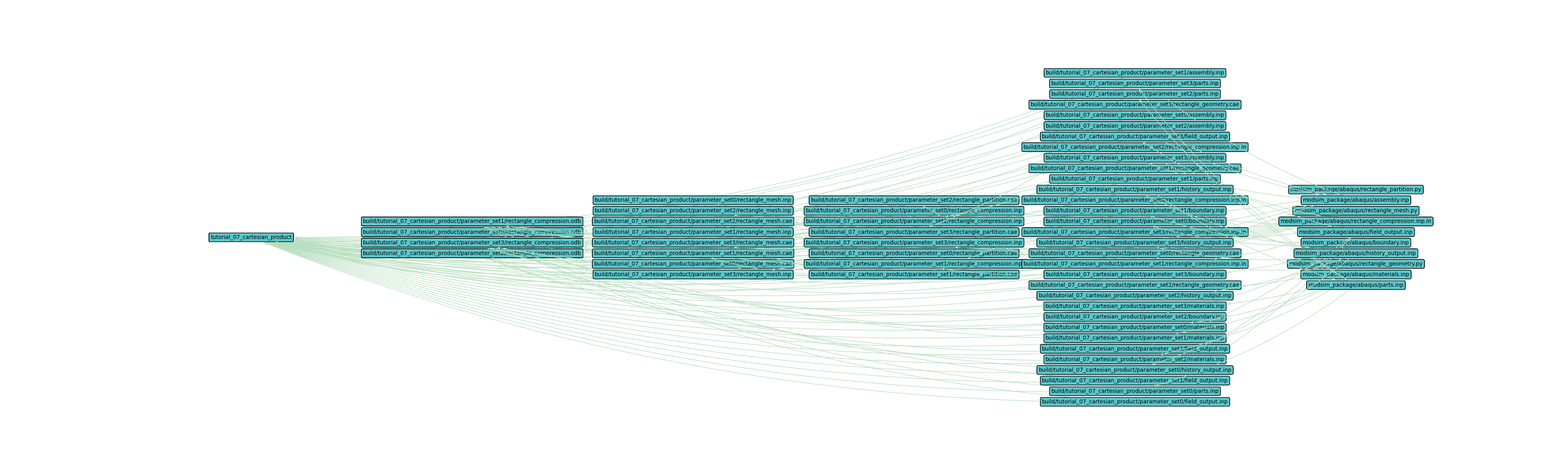
In this figure we begin to see the value of a build system for modsim execution. Despite excluding most of the simulation output files, the full parameter study directed graph is much larger than the one shown in Tutorial 06: Include Files. With the piecewise construction of the input deck standing in for a moderately complex modsim project, even a four set parameter study quickly grows unmanageable for manual state tracking and execution. With SCons managing the directed graph construction, state, and execution, the modsim developer can focus attention on the engineering analysis and benefit from partial re-execution of the parameter study when only a subset of the parameter study has changed.
Now plot the workflow with only the first set, set0.
$ pwd
/home/roppenheimer/waves-tutorials
$ waves visualize tutorial_07_cartesian_product --output-file tutorial_07_cartesian_product_set0.png --width=42 --height=6 --exclude-list /usr/bin .stdout .jnl .prt .com .msg .dat .sta --exclude-regex "set[1-9]"
PS > Get-Location

Path
----
C:\Users\roppenheimer\waves-tutorials

PS > waves visualize tutorial_07_cartesian_product --output-file tutorial_07_cartesian_product_set0.png --width=42 --height=6 --exclude-list .stdout .jnl .prt .com .msg .dat .sta --exclude-regex "set[1-9]"
The output should look similar to the figure below.
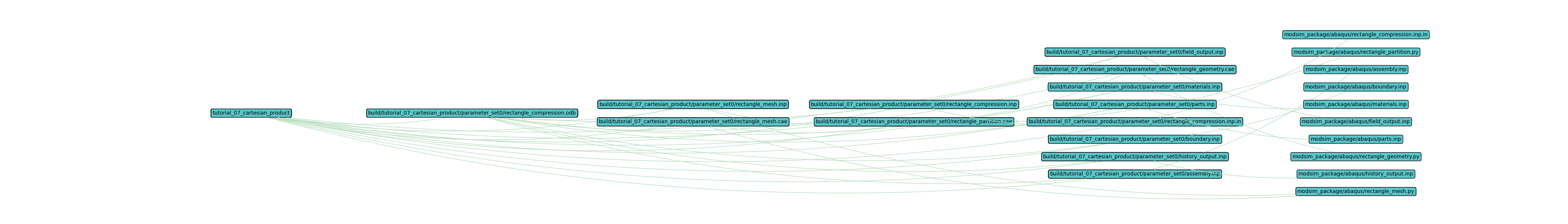
While the first image is useful for demonstrating modsim project size and scope, a more useful directed graph can be
evaluated by limiting the output to a single set. This image should look similar to the
Tutorial 06: Include Files directed graph, but with fewer output files because the *.msg, *.dat, and
*.sta files have been excluded to make the full parameter study graph more readable.