Tutorial: Sensitivity Study#
References#
Environment#
SCons and WAVES can be installed in a Conda environment with the Conda package manager. See the Conda installation and Conda environment management documentation for more details about using Conda.
Note
The SALib and numpy versions may not need to be this strict for most tutorials. However, Tutorial: Sensitivity Study uncovered some undocumented SALib version sensitivity to numpy surrounding the numpy v2 rollout.
Create the tutorials environment if it doesn’t exist
$ conda create --name waves-tutorial-env --channel conda-forge waves 'scons>=4.6' matplotlib pandas pyyaml xarray seaborn 'numpy>=2' 'salib>=1.5.1' pytest
PS > conda create --name waves-tutorial-env --channel conda-forge waves scons matplotlib pandas pyyaml xarray seaborn numpy salib pytest
Activate the environment
$ conda activate waves-tutorial-env
PS > conda activate waves-tutorial-env
Some tutorials require additional third-party software that is not available for the Conda package manager. This
software must be installed separately and either made available to SConstruct by modifying your system’s PATH or by
modifying the SConstruct search paths provided to the waves.scons_extensions.add_program() method.
Warning
STOP! Before continuing, check that the documentation version matches your installed package version.
You can find the documentation version in the upper-left corner of the webpage.
You can find the installed WAVES version with
waves --version.
If they don’t match, you can launch identically matched documentation with the WAVES Command-Line Utility
docs subcommand as waves docs.
Directory Structure#
Create and change to a new project root directory to house the tutorial files if you have not already done so. For example
$ mkdir -p ~/waves-tutorials
$ cd ~/waves-tutorials
$ pwd
/home/roppenheimer/waves-tutorials
PS > New-Item $HOME\waves-tutorials -ItemType "Directory"
PS > Set-Location $HOME\waves-tutorials
PS > Get-Location

Path
----
C:\Users\roppenheimer\waves-tutorials
Note
If you skipped any of the previous tutorials, run the following commands to create a copy of the necessary tutorial files.
$ pwd
/home/roppenheimer/waves-tutorials
$ waves fetch --overwrite --tutorial 12 && mv tutorial_12_archival_SConstruct SConstruct
WAVES fetch
Destination directory: '/home/roppenheimer/waves-tutorials'
Download and copy the
tutorial_12_archival.sconsfile to a new file namedtutorial_sensitivity_study.sconswith the WAVES Command-Line Utility fetch subcommand.
$ pwd
/home/roppenheimer/waves-tutorials
$ waves fetch --overwrite tutorials/tutorial_12_archival.scons && cp tutorial_12_archival.scons tutorial_sensitivity_study.scons
WAVES fetch
Destination directory: '/home/roppenheimer/waves-tutorials'
Parameter Study File#
Create a new file
modsim_package/python/rectangle_compression_sensitivity_study.pyfrom the content below.
waves-tutorials/modsim_package/python/rectangle_compression_sensitivity_study.py
"""Parameter sets and schemas for the rectangle compression simulation."""

import typing


def parameter_schema(
    N: int = 5,  # noqa: N803
    width_distribution: str = "norm",
    width_bounds: list[float] | tuple[float, ...] = (1.0, 0.1),
    height_distribution: str = "norm",
    height_bounds: list[float] | tuple[float, ...] = (1.0, 0.1),
) -> dict[str, typing.Any]:
    """Return WAVES SALibSampler Sobol schema.

    :param N: Number of samples to generate
    :param width_distribution: SALib distribution name
    :param width_bounds: Distribution characteristics. Meaning varies depending on distribution type.
    :param height_distribution: SALib distribution name
    :param height_bounds: Distribution characteristics. Meaning varies depending on distribution type.

    :returns: WAVES SALibSampler Sobol schema
    """
    schema = {
        "N": N,
        "problem": {
            "num_vars": 2,
            "names": ["width", "height"],
            "bounds": [list(width_bounds), list(height_bounds)],
            "dists": [width_distribution, height_distribution],
        },
    }
    return schema
This file should look similar to the parameter study file in Tutorial 07: Sobol Sequence; however, this tutorial uses
the SALib [70] based parameter generator waves.parameter_generators.SALibSampler() instead of the SciPy
[72] based parameter generator waves.parameter_generators.SobolSequence(). Both SALib and SciPy are good
packages for generating samples and post-processing data, but this tutorial will use SALib for the sensitivity analysis
post-processing workflow so the tutorial will generate samples with the matching package. It is not always necessary to
match the sample generator to the sensitivity analysis tools, but some analysis solutions are sensitive to the sample
generation algorithm. Readers are encouraged to review both packages to match the sample generation and analysis
strategy to their needs.
SConscript#
A diff against the tutorial_12_archival.scons file from Tutorial 12: Data Archival is included below to help identify
the changes made in this tutorial.
waves-tutorials/tutorial_sensitivity_study.scons
--- /home/runner/work/waves/waves/build/docs/tutorials_tutorial_12_archival.scons
+++ /home/runner/work/waves/waves/build/docs/tutorials_tutorial_sensitivity_study.scons
@@ -17,7 +17,7 @@

 import waves

-from modsim_package.python.rectangle_compression_cartesian_product import parameter_schema
+from modsim_package.python.rectangle_compression_sensitivity_study import parameter_schema

 # Inherit the parent construction environment
 Import("env")
@@ -27,8 +27,16 @@
 # Simulation variables
 build_directory = pathlib.Path(Dir(".").abspath)
 workflow_name = build_directory.name
-workflow_configuration = [env["project_configuration"], f"{workflow_name}.scons"]
+workflow_configuration = [env["project_configuration"], workflow_name]
 parameter_study_file = build_directory / "parameter_study.h5"
+simulation_constants = {
+    "global_seed": 1,
+    "displacement": -0.01,
+}
+kwargs = {
+    "seed": 42,
+    "calc_second_order": False,
+}

 # Collect the target nodes to build a concise alias for all targets
 workflow = []
@@ -36,11 +44,13 @@

 # Comment used in tutorial code snippets: marker-2

-# Parameter Study with Cartesian Product
-parameter_generator = waves.parameter_generators.CartesianProduct(
+# Parameter Study with SALib Sobol sequence sampler
+parameter_generator = waves.parameter_generators.SALibSampler(
+    "sobol",
     parameter_schema(),
     output_file=parameter_study_file,
     previous_parameter_study=parameter_study_file,
+    **kwargs,
 )
 parameter_generator.write()

@@ -49,7 +59,7 @@
 # Parameterized targets must live inside current simulation_variables for loop
 for set_name, parameters in parameter_generator.parameter_study_to_dict().items():
     set_path = pathlib.Path(set_name)
-    simulation_variables = parameters
+    simulation_variables = {**parameters, **simulation_constants}

     # Comment used in tutorial code snippets: marker-4

@@ -171,26 +181,13 @@
     for set_name in parameter_generator.parameter_study_to_dict()
 ]
 script_options = "--input-file ${SOURCES[2:].abspath}"
-script_options += " --output-file ${TARGET.file} --x-units mm/mm --y-units MPa"
+script_options += " --output-file ${TARGET.file}"
 script_options += " --parameter-study-file ${SOURCES[1].abspath}"
 workflow.extend(
     env.PythonScript(
-        target=["stress_strain_comparison.pdf", "stress_strain_comparison.csv"],
-        source=["#/modsim_package/python/post_processing.py", parameter_study_file.name, *post_processing_source],
+        target=["sensitivity_study.pdf", "sensitivity_study.csv", "sensitivity_study.yaml"],
+        source=["#/modsim_package/python/sensitivity_study.py", parameter_study_file.name, *post_processing_source],
         subcommand_options=script_options,
-    )
-)
-
-# Regression test
-workflow.extend(
-    env.PythonScript(
-        target=["regression.yaml"],
-        source=[
-            "#/modsim_package/python/regression.py",
-            "stress_strain_comparison.csv",
-            "#/modsim_package/python/rectangle_compression_cartesian_product.csv",
-        ],
-        subcommand_options="${SOURCES[1:].abspath} --output-file ${TARGET.abspath}",
     )
 )

@@ -206,15 +203,10 @@
 env.Alias(f"{workflow_name}_datacheck", datacheck)
 env.Alias(env["datacheck_alias"], datacheck)
 env.Alias(env["regression_alias"], datacheck)
-archive_alias = f"{workflow_name}_archive"
-env.Alias(archive_alias, archive_target)
+env.Alias(f"{workflow_name}_archive", archive_target)

 if not env["unconditional_build"] and not env["ABAQUS_PROGRAM"]:
-    print(
-        "Program 'abaqus' was not found in construction environment."
-        f" Ignoring '{workflow_name}' and '{archive_alias}' target(s)"
-    )
+    print(f"Program 'abaqus' was not found in construction environment. Ignoring '{workflow_name}' target(s)")
     Ignore([".", workflow_name], workflow)
-    Ignore([".", archive_alias], archive_target)
     Ignore([".", f"{workflow_name}_datacheck"], datacheck)
     Ignore([".", env["datacheck_alias"], env["regression_alias"]], datacheck)
Post-processing script#
In the
waves-tutorials/modsim_package/pythondirectory, create a file calledsensitivity_study.pyusing the contents below.
waves-tutorials/modsim_package/python/sensitivity_study.py
#!/usr/bin/env python
"""Example of catenating WAVES parameter study results and definition."""

import argparse
import pathlib
import sys

import matplotlib.pyplot
import numpy
import pandas
import SALib.analyze.delta
import seaborn
import xarray
import yaml
from waves.parameter_generators import SET_COORDINATE_KEY

from modsim_package.python.rectangle_compression_sensitivity_study import parameter_schema

default_selection_dict = {
    "E values": "E22",
    "S values": "S22",
    "elements": 1,
    "step": "Step-1",
    "time": 1.0,
    "integration point": 0,
}


def combine_data(
    input_files: list[str | pathlib.Path],
    group_path: str,
    concat_coord: str,
) -> xarray.Dataset:
    """Combine input data files into one dataset.

    :param input_files: list of path-like or file-like objects pointing to h5netcdf files
        containing Xarray Datasets
    :param group_path: The h5netcdf group path locating the Xarray Dataset in the input files.
    :param concat_coord: Name of dimension

    :returns: Combined data
    """
    paths = [pathlib.Path(input_file).resolve() for input_file in input_files]
    data_generator = (
        xarray.open_dataset(path, group=group_path, engine="h5netcdf").assign_coords({concat_coord: path.parent.name})
        for path in paths
    )
    combined_data = xarray.concat(data_generator, concat_coord, join="outer", compat="no_conflicts")
    combined_data.close()

    return combined_data


def merge_parameter_study(
    parameter_study_file: str | pathlib.Path,
    combined_data: xarray.Dataset,
) -> xarray.Dataset:
    """Merge parameter study to existing dataset.

    :param parameter_study_file: path-like or file-like object containing the parameter study dataset. Assumes the
        h5netcdf file contains only a single dataset at the root group path, .e.g. ``/``.
    :param combined_data: XArray Dataset that will be merged.

    :returns: Combined data
    """
    parameter_study = xarray.open_dataset(parameter_study_file, engine="h5netcdf")
    combined_data = combined_data.merge(parameter_study)
    parameter_study.close()
    return combined_data


def main(
    input_files: list[pathlib.Path],
    output_file: pathlib.Path,
    group_path: str,
    selection_dict: dict,
    parameter_study_file: pathlib.Path | None = None,
) -> None:
    """Catenate ``input_files`` datasets along the ``set_name`` dimension and plot selected data.

    Merges the parameter study results datasets with the parameter study definition dataset, where the parameter study
    dataset file is assumed to be written by a WAVES parameter generator.

    :param list input_files: list of path-like or file-like objects pointing to h5netcdf files containing Xarray
        Datasets
    :param str output_file: The correlation coefficients plot file name. Relative or absolute path.
    :param str group_path: The h5netcdf group path locating the Xarray Dataset in the input files.
    :param dict selection_dict: Dictionary to define the down selection of data to be plotted. Dictionary ``key: value``
        pairs must match the data variables and coordinates of the expected Xarray Dataset object.
    :param str parameter_study_file: path-like or file-like object containing the parameter study dataset. Assumes the
        h5netcdf file contains only a single dataset at the root group path, .e.g. ``/``.
    """
    output_file = pathlib.Path(output_file)
    output_csv = output_file.with_suffix(".csv")
    output_yaml = output_file.with_suffix(".yaml")
    concat_coord = SET_COORDINATE_KEY

    # Build single dataset along the "set_name" dimension
    combined_data = combine_data(input_files, group_path, concat_coord)

    # Merge WAVES parameter study if provided
    combined_data = merge_parameter_study(parameter_study_file, combined_data)

    # Correlation coefficients
    correlation_data = combined_data.sel(selection_dict).to_array().to_pandas().transpose()
    seaborn.pairplot(correlation_data, corner=True)
    matplotlib.pyplot.savefig(output_file)

    correlation_matrix = numpy.corrcoef(correlation_data.to_numpy(), rowvar=False)
    correlation_coefficients = pandas.DataFrame(
        correlation_matrix, index=correlation_data.columns, columns=correlation_data.columns
    )
    correlation_coefficients.to_csv(output_csv)

    # Sensitivity analysis
    stress = combined_data.sel(selection_dict)["S"].to_numpy()
    inputs = combined_data.sel(selection_dict)[["width", "height"]].to_array().transpose().to_numpy()
    sensitivity = SALib.analyze.delta.analyze(parameter_schema()["problem"], inputs, stress)
    sensitivity_yaml = {}
    for key, value in sensitivity.items():
        if isinstance(value, numpy.ndarray):
            yaml_compatible_value = value.tolist()
        else:
            yaml_compatible_value = value
        sensitivity_yaml[key] = yaml_compatible_value
    with output_yaml.open(mode="w") as output:
        output.write(yaml.safe_dump(sensitivity_yaml))

    # Clean up open files
    combined_data.close()


def get_parser() -> argparse.ArgumentParser:
    """Return parser for CLI options."""
    script_name = pathlib.Path(__file__)
    default_output_file = f"{script_name.stem}.pdf"
    default_group_path = "RECTANGLE/FieldOutputs/ALL_ELEMENTS"
    default_parameter_study_file = None

    prog = f"python {script_name.name} "
    cli_description = (
        "Read Xarray Datasets and plot correlation coefficients as a function of parameter set name. "
        " Save to ``output_file``."
    )
    parser = argparse.ArgumentParser(description=cli_description, prog=prog)
    required_named = parser.add_argument_group("required named arguments")
    required_named.add_argument(
        "-i",
        "--input-file",
        nargs="+",
        type=pathlib.Path,
        required=True,
        help="The Xarray Dataset file(s)",
    )
    required_named.add_argument(
        "-p",
        "--parameter-study-file",
        type=pathlib.Path,
        default=default_parameter_study_file,
        help="An optional h5 file with a WAVES parameter study Xarray Dataset (default: %(default)s)",
    )

    parser.add_argument(
        "-o",
        "--output-file",
        type=pathlib.Path,
        default=default_output_file,
        help=(
            "The output file for the correlation coefficients plot with extension, "
            "e.g. ``output_file.pdf``. Extension must be supported by matplotlib. File stem is also "
            "used for the CSV table output, e.g. ``output_file.csv``, and sensitivity results, e.g. "
            "``output_file.yaml``. (default: %(default)s)"
        ),
    )
    parser.add_argument(
        "-g",
        "--group-path",
        type=str,
        default=default_group_path,
        help="The h5py group path to the dataset object (default: %(default)s)",
    )
    parser.add_argument(
        "-s",
        "--selection-dict",
        type=pathlib.Path,
        default=None,
        help=(
            "The YAML formatted dictionary file to define the down selection of data to be plotted. "
            "Dictionary key: value pairs must match the data variables and coordinates of the "
            "expected Xarray Dataset object. If no file is provided, the a default selection dict "
            f"will be used (default: {default_selection_dict})"
        ),
    )

    return parser


if __name__ == "__main__":
    parser = get_parser()
    args = parser.parse_args()
    if not args.selection_dict:
        selection_dict = default_selection_dict
    else:
        with args.selection_dict.open(mode="r") as input_yaml:
            selection_dict = yaml.safe_load(input_yaml)
    sys.exit(
        main(
            input_files=args.input_file,
            output_file=args.output_file,
            group_path=args.group_path,
            selection_dict=selection_dict,
            parameter_study_file=args.parameter_study_file,
        )
    )
This file should look similar to the post_processing.py file from Tutorial 09: Post-Processing. Unused functions
have been removed and the output has changed to reflect the sensitivity study operations. In practice, modsim projects
should move the shared functions of both post-processing scripts to a common utilities module.
Unlike Tutorial 09: Post-Processing, the sensitivity study script does require the parameter study file. It is not possible to calculate the sensitivity of output variables to input variables without associating output files with their parameter set. After merging the output datasets with the parameter study, the correlation coefficients can be plotted with seaborn [71]. Numpy [69] is used to perform a similar correlation coefficients calculation that can be saved to a CSV file for further post-processing or regression testing as in Tutorial 11: Regression Testing. Finally, SALib [70] is used to perform a delta moment-independent analysis, which is compatible with all SALib sampling techniques.
The value of processing output data into an Xarray [46] dataset is evident here, where each new plotting and analysis tool requires data in a slightly different form factor. For these tutorials, WAVES provides an extraction utility to process simulation output data into an Xarray dataset. However, it is well worth the modsim owner’s time to seek out or write similar data serialization utilities for all project numeric solvers. Beyond the ease of post-processing, tightly coupled and named column data structures reduce the chances of post-processing errors during data handling operations.
While the post-processing approach outlined in this tutorial gives users a starting point for performing all forms of parameter studies (sensitivity, perturbation, uncertainty propagation, etc) the choice of input sampling tools, parameter sampling ranges and distributions, and analysis tools is highly dependent on the needs of the project and the characteristics of the input space and numerical solvers. Modsim project owners are encouraged to read the sampling and analysis documentation closely and seek advice from statistics and uncertainty experts in building and interpreting their parameter studies.
SConstruct#
Update the
SConstructfile. Adiffagainst theSConstructfile from Tutorial 12: Data Archival is included below to help identify the changes made in this tutorial.
waves-tutorials/SConstruct
--- /home/runner/work/waves/waves/build/docs/tutorials_tutorial_12_archival_SConstruct
+++ /home/runner/work/waves/waves/build/docs/tutorials_tutorial_sensitivity_study_SConstruct
@@ -1,5 +1,5 @@
 #! /usr/bin/env python
-"""Configure the WAVES archive tutorial."""
+"""Configure the WAVES sensitivity analysis tutorial."""

 import inspect
 import os
@@ -122,6 +122,7 @@
     "tutorial_09_post_processing.scons",
     "tutorial_11_regression_testing.scons",
     "tutorial_12_archival.scons",
+    "tutorial_sensitivity_study.scons",
 ]
 for workflow in workflow_configurations:
     build_dir = env["variant_dir_base"] / pathlib.Path(workflow).stem
Build Targets#
Build the new sensitivity study targets
$ pwd
/home/roppenheimer/waves-tutorials
$ scons tutorial_sensitivity_study --jobs=4
<output truncated>
Output Files#
Explore the contents of the build directory using the tree command against the build directory, as shown
below. Note that the output files from the previous tutorials may also exist in the build directory, but the
directory is specified by name to reduce clutter in the output shown.
$ pwd
/home/roppenheimer/waves-tutorials
$ tree build/tutorial_sensitivity_study/ -L 1
build/tutorial_sensitivity_study/
|-- correlation_pairplot.pdf
|-- parameter_set0
|-- parameter_set1
|-- parameter_set10
|-- parameter_set11
|-- parameter_set12
|-- parameter_set13
|-- parameter_set14
|-- parameter_set15
|-- parameter_set16
|-- parameter_set17
|-- parameter_set18
|-- parameter_set19
|-- parameter_set2
|-- parameter_set3
|-- parameter_set4
|-- parameter_set5
|-- parameter_set6
|-- parameter_set7
|-- parameter_set8
|-- parameter_set9
|-- parameter_study.h5
|-- sensitivity.yaml
|-- sensitivity_study.csv
`-- sensitivity_study.csv.stdout

20 directories, 5 files
The purpose of the sensitivity study is to observe the relationships between the input space parameters (width and height) on the output space parameters (peak stress). The script writes a correlation coefficients plot relating each input and output space parameter to every other parameter.
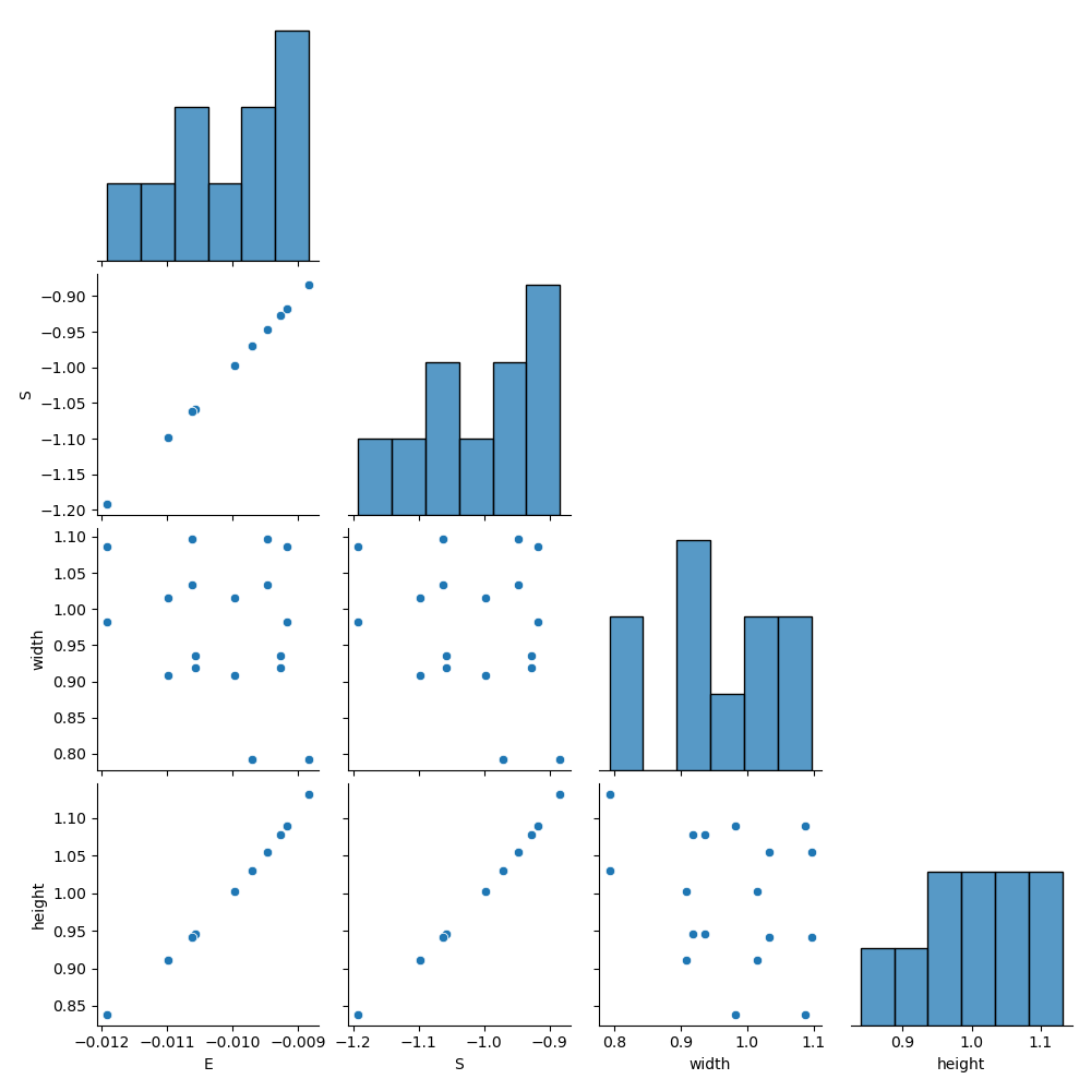
Correlation coefficients#
In the Correlation coefficients figure we can see both the input and output histograms on the diagonal. The scatter plots show the relationships between parameters. We can see very little correlation between the stress output and the width input, and strongly linear correlation between the stress output and the height input. This is the result we should expect because we are applying a fixed displacement load and stress is linearly dependent on the applied strain, which is a function of the change in displacement and the unloaded height. If we were instead applying a force, we should expect the opposite correlation because stress would then depend on the applied load divided by the cross-sectional area.