Quickstart

Quickstart#

This quickstart will create a minimal, two file project configuration combining elements of the tutorials listed below.

These tutorials and this quickstart describe the computational engineering workflow through simulation execution and post-processing. This tutorial will use a different working directory and directory structure than the rest of the tutorials to avoid filename clashes. The quickstart also uses a flat directory structure to simplify the project configuration. Larger projects, like the ModSim Templates, may require a hierarchical directory structure to separate files with identical basenames.

Environment#

SCons and WAVES can be installed in a Conda environment with the Conda package manager. See the Conda installation and Conda environment management documentation for more details about using Conda.

Note

The SALib and numpy versions may not need to be this strict for most tutorials. However, Tutorial: Sensitivity Study uncovered some undocumented SALib version sensitivity to numpy surrounding the numpy v2 rollout.

Create the tutorials environment if it doesn’t exist

$ conda create --name waves-tutorial-env --channel conda-forge waves 'scons>=4.6' matplotlib pandas pyyaml xarray seaborn 'numpy>=2' 'salib>=1.5.1' pytest

Activate the environment
```
$ conda activate waves-tutorial-env
```

Some tutorials require additional third-party software that is not available for the Conda package manager. This software must be installed separately and either made available to SConstruct by modifying your system’s PATH or by modifying the SConstruct search paths provided to the waves.scons_extensions.add_program() method.

Warning

STOP! Before continuing, check that the documentation version matches your installed package version.

You can find the documentation version in the upper-left corner of the webpage.
You can find the installed WAVES version with waves --version.

If they don’t match, you can launch identically matched documentation with the WAVES Command-Line Utility docs subcommand as waves docs.

Directory Structure#

Create the project directory structure and copy the WAVES quickstart source files into the ~/waves-tutorials/waves_quickstart sub-directory with the WAVES Command-Line Utility fetch subcommand.

$ waves fetch tutorials/waves_quickstart --destination ~/waves-tutorials/waves_quickstart
WAVES fetch
Destination directory: '/home/roppenheimer/waves-tutorials/waves_quickstart'
$ cd ~/waves-tutorials/waves_quickstart
$ pwd
/home/roppenheimer/waves-tutorials/waves_quickstart

SConscript#

Managing digital data and workflows in modern computational science and engineering is a difficult and error-prone task. The large number of steps in the workflow and complex web of interactions between data files results in non-intuitive dependencies that are difficult to manage by hand. This complexity grows substantially when the workflow includes parameter studies. WAVES enables the use of traditional software build systems in computational science and engineering workflows with support for common engineering software and parameter study management.

Build systems construct a directed acyclic graph (DAG) from small, individual task definitions. Each task is defined by the developer and subsequently linked by the build system. Tasks are composed of targets, sources, and actions. A target is the output of the task. Sources are the required direct-dependency files used by the task and may be files tracked by the version control system for the project or files produced by other tasks. Actions are the executable commands that produce the target files. In pseudocode, this might look like a dictionary:

task1:
    target: output1
    source: source1
    action: action1 --input source1 --output output1

task2:
    target: output2
    source: output1
    action: action2 --input output1 --output output2

As the number of discrete tasks increases, and as cross-dependencies grow, an automated tool to construct the build order becomes more important. Besides simplifying the process of constructing the workflow DAG, most build systems also incorporate a state machine. The build system tracks the execution state of the DAG and will only re-build out-of-date portions of the DAG. This is especially valuable when trouble-shooting or expanding a workflow. For instance, when adding or modifying the post-processing step, the build system will not re-run simulation tasks that are computationally expensive and require significant wall time to solve.

The SConscript file below contains the workflow task definitions. Review the source and target files defining the workflow tasks. As discussed briefly above and in detail in Build System, a task definition also requires an action. For convenience, WAVES provides builders for common engineering software with pre-defined task actions. See the waves.scons_extensions.abaqus_journal_builder_factory() and waves.scons_extensions.abaqus_solver_builder_factory() for more complete descriptions of the builder actions.

waves_quickstart/SConscript

Import("env", "alias", "parameters")

# Geometry
env.AbaqusJournal(
    target=["rectangle_geometry.cae", "rectangle_geometry.jnl"],
    source=["rectangle_geometry.py"],
    subcommand_options="--width ${width} --height ${height}",
    **parameters,
)

# Partition
env.AbaqusJournal(
    target=["rectangle_partition.cae", "rectangle_partition.jnl"],
    source=["rectangle_partition.py", "rectangle_geometry.cae"],
    subcommand_options="--width ${width} --height ${height}",
    **parameters,
)

# Mesh
env.AbaqusJournal(
    target=["rectangle_mesh.inp", "rectangle_mesh.cae", "rectangle_mesh.jnl"],
    source=["rectangle_mesh.py", "rectangle_partition.cae", "abaqus_utilities.py"],
    subcommand_options="--global-seed ${global_seed}",
    **parameters,
)

# SolverPrep
env.CopySubstfile(
    ["#/rectangle_compression.inp.in"],
    substitution_dictionary=env.SubstitutionSyntax(parameters),
)

# Abaqus Solve
env.AbaqusStandard(
    target=["rectangle_compression.odb"],
    source=["rectangle_compression.inp"],
    job="rectangle_compression",
    program_options="-double both",
    **parameters,
)

# Abaqus Extract
env.AbaqusExtract(
    target=["rectangle_compression.h5", "rectangle_compression_datasets.h5"],
    source=["rectangle_compression.odb"],
)

# Post-processing
target = env.PythonScript(
    target=["stress_strain.pdf", "stress_strain.csv"],
    source=["post_processing.py", "rectangle_compression_datasets.h5"],
    subcommand_options="--input-file ${SOURCES[1:].abspath} --output-file ${TARGET.file} --x-units mm/mm --y-units MPa",
)

# Collector alias named after the model simulation
env.Alias(alias, target)

if not env["unconditional_build"] and not env["ABAQUS_PROGRAM"]:
    print(f"Program 'abaqus' was not found in construction environment. Ignoring 'rectangle' target(s)")
    Ignore([".", alias], target)

SConstruct#

For this quickstart, we will not discuss the main SCons configuration file, named SConstruct, in detail. Tutorial 00: SConstruct has a more complete discussion about the contents of the SConstruct file.

One of the primary benefits to WAVES is the ability to robustly integrate the conditional re-building behavior of a build system with computational parameter studies. Because most build systems consist of exactly two steps: configuration and execution, the full DAG must be fixed at configuration time. To avoid hardcoding the parameter study tasks, it is desirable to re-use the existing workflow or task definitions. This could be accomplished with a simple for-loop and naming convention; however, it is common to run a small, scoping parameter study prior to exploring the full parameter space which would require careful set re-numbering to preserve previous work.

To avoid out-of-sync errors in parameter set definitions when updating a previously executed parameter study, WAVES provides a parameter study generator utility that uniquely identifies parameter sets by contents, assigns a unique index to each parameter set, and guarantees that previously executed sets are matched to their unique identifier. When expanding or re-executing a parameter study, WAVES enforces set name/content consistency which in turn ensures that the build system can correctly identify previous work and only re-build the new or changed sets.

In the configuration snippet below, the workflow parameterization is performed in the root configuration file, SConstruct. This allows us to re-use the entire workflow file, SConscript, with more than one parameter study. First, we define a nominal workflow. Nominal workflows can be defined as a simple dictionary. This can be useful for trouble-shooting the workflow, simulation definition, and simulation convergence prior to running a larger parameter study. Second, we define a small mesh convergence study where the only parameter that changes is the mesh global seed.

waves_quickstart/SConstruct

# Define parameter studies
nominal_parameters = {
    "width": 1.0,
    "height": 1.0,
    "global_seed": 1.0,
    "displacement": -0.01,
}
mesh_convergence_parameter_study_file = env["parameter_study_directory"] / "mesh_convergence.h5"
mesh_convergence_parameter_generator = waves.parameter_generators.CartesianProduct(
    {
        "width": [1.0],
        "height": [1.0],
        "global_seed": [1.0, 0.5, 0.25, 0.125],
        "displacement": [-0.01],
    },
    output_file=mesh_convergence_parameter_study_file,
    previous_parameter_study=mesh_convergence_parameter_study_file,
)
mesh_convergence_parameter_generator.write()

Finally, we call the workflow SConscript file in a loop where the study names and definitions are unpacked into the workflow call. The ParameterStudySConscript method handles the differences between a nominal parameter set dictionary and the mesh convergence parameter study object. The SConscript file has been written to accept the parameters variable that will be unpacked by this function.

waves_quickstart/SConstruct

# Add workflow(s)
workflow_configurations = [
    ("nominal", nominal_parameters),
    ("mesh_convergence", mesh_convergence_parameter_generator),
]
for study_name, study_definition in workflow_configurations:
    env.ParameterStudySConscript(
        "SConscript",
        variant_dir=env["build_dir"] / study_name,
        exports={"env": env, "alias": study_name},
        study=study_definition,
        subdirectories=True,
        duplicate=True,
    )

In this tutorial, the entire workflow is re-run from scratch for each parameter set. This simplifies the parameter study construction and enables the geometric parameterization hinted at in the width and height parameters. Not all workflows require the same level of granularity and re-use. There are resource trade-offs to workflow construction, task definition granularity, and computational resources. For instance, if the geometry and partition tasks required significant wall time, but are not part of the mesh convergence study, it might be desirable to parameterize within the SConscript file where the geometry and partition tasks could be excluded from the parameter study.

WAVES provides several solutions for parameterizing at the level of workflow files, task definitions, or in arbitrary locations and methods, depending on the needs of the project.

workflow files: waves.scons_extensions.parameter_study_sconscript()
task definitions: waves.scons_extensions.parameter_study_task()
anywhere: waves.parameter_generators.ParameterGenerator.parameter_study_to_dict()

Building targets#

Note

You may need to pass the relative or absolute path to your Abaqus installation when running the workflow.

scons --abaqus-command /path/to/executable/abaqus ...

You can also edit the SConstruct file contents below to include your Abaqus installation in the default search for an Abaqus executable.

waves_quickstart/SConstruct

default_abaqus_commands = [
    "/apps/abaqus/Commands/abq2024",
    "/usr/projects/ea/abaqus/Commands/abq2024",
    "abq2024",
    "abaqus",
]

The waves.scons_extensions.WAVESEnvironment.AddProgram() method performs an ordered preference search for executables by absolute and relative paths in the system PATH.

In SConstruct, the workflows were provided aliases matching the study names for more convenient execution. First, run the nominal workflow and observe the task command output as below. The default behavior of SCons is to report each task’s action as it is executed. WAVES builders capture the STDOUT and STDERR into per-task log files to aid in troubleshooting and to remove clutter from the terminal output. On first execution you may see a warning message as a previous parameter study is being requested which will only exist on subsequent executions.

$ pwd
/home/roppenheimer/waves-tutorials/waves_quickstart
$ scons nominal
scons: Reading SConscript files ...
Checking whether '/apps/abaqus/Commands/abq2024' program exists.../apps/abaqus/Commands/abq2024
Checking whether '/usr/projects/ea/abaqus/Commands/abq2024' program exists...no
Checking whether 'abq2024' program exists...no
Checking whether 'abaqus' program exists...no
scons: done reading SConscript files.
scons: Building targets ...
Copy("build/nominal/rectangle_compression.inp.in", "rectangle_compression.inp.in")
Creating 'build/nominal/rectangle_compression.inp'
cd /home/roppenheimer/waves-tutorials/waves_quickstart/build/nominal && /apps/abaqus/Commands/abq2024 cae -noGUI /home/roppenheimer/waves-tutorials/waves_quickstart/build/nominal/rectangle_geometry.py -- --width 1.0 --height 1.0 > /home/roppenheimer/waves-tutorials/waves_quickstart/build/nominal/rectangle_geometry.cae.stdout 2>&1
cd /home/roppenheimer/waves-tutorials/waves_quickstart/build/nominal && /apps/abaqus/Commands/abq2024 cae -noGUI /home/roppenheimer/waves-tutorials/waves_quickstart/build/nominal/rectangle_partition.py -- --width 1.0 --height 1.0 > /home/roppenheimer/waves-tutorials/waves_quickstart/build/nominal/rectangle_partition.cae.stdout 2>&1
cd /home/roppenheimer/waves-tutorials/waves_quickstart/build/nominal && /apps/abaqus/Commands/abq2024 cae -noGUI /home/roppenheimer/waves-tutorials/waves_quickstart/build/nominal/rectangle_mesh.py -- --global-seed 1.0 > /home/roppenheimer/waves-tutorials/waves_quickstart/build/nominal/rectangle_mesh.inp.stdout 2>&1
cd /home/roppenheimer/waves-tutorials/waves_quickstart/build/nominal && /apps/abaqus/Commands/abq2024 -interactive -ask_delete no -job rectangle_compression -input rectangle_compression -double both > /home/roppenheimer/waves-tutorials/waves_quickstart/build/nominal/rectangle_compression.stdout 2>&1
_build_odb_extract(["build/nominal/rectangle_compression.h5", "build/nominal/rectangle_compression_datasets.h5", "build/nominal/rectangle_compression.csv"], ["build/nominal/rectangle_compression.odb"])
cd /home/roppenheimer/waves-tutorials/waves_quickstart/build/nominal && python /home/roppenheimer/waves-tutorials/waves_quickstart/build/nominal/post_processing.py --input-file /home/roppenheimer/waves-tutorials/waves_quickstart/build/nominal/rectangle_compression_datasets.h5 --output-file stress_strain.pdf --x-units mm/mm --y-units MPa > /home/roppenheimer/waves-tutorials/waves_quickstart/build/nominal/stress_strain.pdf.stdout 2>&1
scons: done building targets.

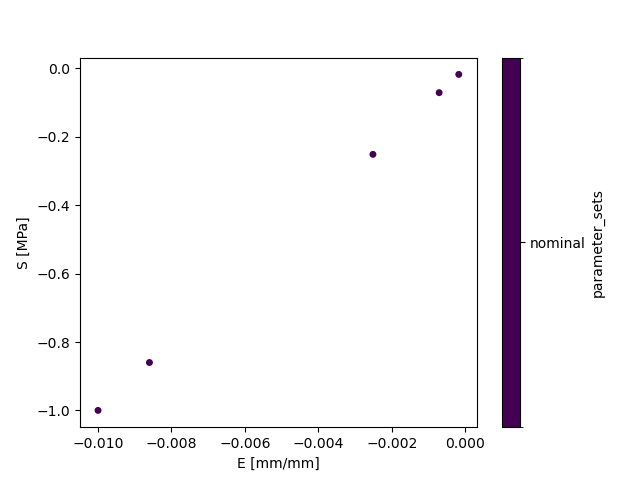
You will find the output files in the build directory. The final post-processing image of the uniaxial compression stress-strain curve is found in stress_strain.pdf.

$ pwd
/home/roppenheimer/waves-tutorials/waves_quickstart
$ ls build/nominal/stress_strain.pdf
build/nominal/stress_strain.pdf

_images/waves_quickstart_stress_strain.png

Before running the parameter study, explore the conditional re-build behavior of the workflow by deleting the intermediate output file rectangle_mesh.inp and re-executing the workflow. You should observe that only the command which produces the orphan mesh rectangle_mesh.inp file is re-run. You can confirm by inspecting the time stamps of files in the build directory before and after file removal and workflow execution.

$ pwd
/home/roppenheimer/waves-tutorials/waves_quickstart
$ rm build/nominal/rectangle_mesh.inp
$ scons nominal
scons: Reading SConscript files ...
Checking whether '/apps/abaqus/Commands/abq2024' program exists.../apps/abaqus/Commands/abq2024
Checking whether '/usr/projects/ea/abaqus/Commands/abq2024' program exists...no
Checking whether 'abq2024' program exists...no
Checking whether 'abaqus' program exists...no
scons: done reading SConscript files.
scons: Building targets ...
cd /home/roppenheimer/waves-tutorials/waves_quickstart/build/nominal && /apps/abaqus/Commands/abq2024 cae -noGUI /home/roppenheimer/waves-tutorials/waves_quickstart/build/nominal/rectangle_mesh.py -- --global-seed 1.0 > /home/roppenheimer/waves-tutorials/waves_quickstart/build/nominal/rectangle_mesh.inp.stdout 2>&1
scons: `nominal' is up to date.
scons: done building targets.

You should expect that the geometry and partition tasks do not need to re-execute because their output files still exist and they are upstream of the mesh task. But the tasks after the mesh task did not re-execute, either. This should be somewhat surprising. The simulation itself depends on the mesh file, so why didn’t the workflow re-execute all tasks from mesh to post-processing?

Many software build systems, such as GNU Make use file system modification time stamps to track DAG state. By default the SCons state machine uses file signatures built from md5 hashes to identify task state. If the contents of the rectangle_mesh.inp file do not change, then the md5 signature on re-execution still matches the build state for the rest of the downstream tasks, which do not need to rebuild.

This default behavior of SCons makes it desirable for computational science and engineering workflows where downstream tasks may be computationally expensive. The added cost of computing md5 signatures during configuration is valuable if it prevents re-execution of a computationally expensive simulation. In actual practice, production engineering analysis workflows may include tasks and simulations with wall clock run times of hours to days. By comparison, the cost of using md5 signatures instead of time stamps is often negligible.

Now run the mesh convergence study as below. SCons uses the --jobs option to control the number of threads used in task execution and will run up to 4 tasks simultaneously.

$ pwd
/home/roppenheimer/waves-tutorials/waves_quickstart
$ scons mesh_convergence --jobs=4
...

The output is truncated, but should look very similar to the nominal output above, where the primary difference is that each parameter set is nested one directory lower using the parameter set number.

$ pwd
/home/roppenheimer/waves-tutorials/waves_quickstart
$ ls build/mesh_convergence/
parameter_set0/  parameter_set1/  parameter_set2/  parameter_set3/

These set names are managed by the WAVES parameter study object, which is written to a separate build directory for later re-execution. This parameter study file is used in the parameter study object construction to identify previously created parameter sets on re-execution.

$ pwd
/home/roppenheimer/waves-tutorials/waves_quickstart
$ ls build/parameter_studies/
mesh_convergence.h5
$ waves print_study build/parameter_studies/mesh_convergence.h5
                                        set_hash  width  height  global_seed  displacement
set_name
parameter_set0  cf0934b22f43400165bd3d34aa61013f    1.0     1.0        1.000         -0.01
parameter_set1  ee7d06f97e3dab5010007d57b2a4ee45    1.0     1.0        0.500         -0.01
parameter_set2  93de452cc9564a549338e87ad98e5288    1.0     1.0        0.250         -0.01
parameter_set3  49e34595c98442a228efd9e9765f61dd    1.0     1.0        0.125         -0.01

Try adding a new global mesh seed in the middle of the existing range. An example might look like the following, where the seed 0.4 is added between 0.5 and 0.25.

SConstruct#

mesh_convergence_parameter_generator = waves.parameter_generators.CartesianProduct(
     {
        "width": [1.0],
        "height": [1.0],
        "global_seed": [1.0, 0.5, 0.4, 0.25, 0.125],
        "displacement": [-0.01],
    },
    output_file=mesh_convergence_parameter_study_file,
    previous_parameter_study=mesh_convergence_parameter_study_file
)

Then re-run the parameter study. The new parameter set should build under the name parameter_set4 and workflow should build only parameter_set4 tasks. The parameter study file should also be updated in the build directory.

$ pwd
/home/roppenheimer/waves-tutorials/waves_quickstart
$ scons mesh_convergence --jobs=4
$ ls build/mesh_convergence/
parameter_set0/  parameter_set1/  parameter_set2/  parameter_set3/ parameter_set4/
$ waves print_study build/parameter_studies/mesh_convergence.h5
                                        set_hash  width  height  global_seed  displacement
set_name
parameter_set0  cf0934b22f43400165bd3d34aa61013f    1.0     1.0        1.000         -0.01
parameter_set1  ee7d06f97e3dab5010007d57b2a4ee45    1.0     1.0        0.500         -0.01
parameter_set2  93de452cc9564a549338e87ad98e5288    1.0     1.0        0.250         -0.01
parameter_set3  49e34595c98442a228efd9e9765f61dd    1.0     1.0        0.125         -0.01
parameter_set4  4a49100665de0220143675c0d6626c50    1.0     1.0        0.400         -0.01

If the parameter study naming convention were managed by hand it would likely be necessary to add the new seed to the end of the parameter study to guarantee that the new set received a new set number. In practice, parameter studies are often defined programmatically as a range() or vary more than one parameter, which makes it difficult to predict how the set numbers may change. It would be tedious and error-prone to re-number the parameter sets such that the input/output relationships are consistent. In the best case, mistakes in set re-numbering would result in unnecessary re-execution of the previous parameter sets. In the worst case, mistakes could result in silent inconsistencies in the input/output relationships and lead to errors in result interpretations.

WAVES first looks for and opens the previous parameter study file saved in the build directory, reads the previous set definitions if the file exists, and then merges the previous study definition with the current definition along the unique set contents identifier coordinate. Under the hood, this unique identifier is an md5 hash of a string representation of the set contents, which is robust between systems with identical machine precision. To avoid long, unreadable hashes in build system paths, the unique md5 hashes are tied to the more human readable set numbers seen in the mesh convergence build directory.

Output Files#

An example of the full nominal workflow output files is found below using the tree command. If tree is not installed on your system, you can use the find command as find build/nominal -type f. If you run a similar command against the mesh convergence build directory you should see the same set of files repeated once per parameter set because the workflow definitions are identical for each parameter set.

$ pwd
/home/roppenheimer/waves-tutorials/waves_quickstart
$ tree build/nominal
build/nominal
|-- SConscript
|-- abaqus.rpy
|-- abaqus.rpy.1
|-- abaqus.rpy.2
|-- abaqus_utilities.py
|-- abaqus_utilities.pyc
|-- post_processing.py
|-- rectangle_compression.com
|-- rectangle_compression.csv
|-- rectangle_compression.dat
|-- rectangle_compression.h5
|-- rectangle_compression.inp
|-- rectangle_compression.inp.in
|-- rectangle_compression.msg
|-- rectangle_compression.odb
|-- rectangle_compression.prt
|-- rectangle_compression.sta
|-- rectangle_compression.stdout
|-- rectangle_compression_datasets.h5
|-- rectangle_geometry.cae
|-- rectangle_geometry.cae.stdout
|-- rectangle_geometry.jnl
|-- rectangle_geometry.py
|-- rectangle_mesh.cae
|-- rectangle_mesh.inp
|-- rectangle_mesh.inp.stdout
|-- rectangle_mesh.jnl
|-- rectangle_mesh.py
|-- rectangle_partition.cae
|-- rectangle_partition.cae.stdout
|-- rectangle_partition.jnl
|-- rectangle_partition.py
|-- stress_strain.csv
|-- stress_strain.pdf
`-- stress_strain.pdf.stdout

0 directories, 35 files

Workflow Visualization#

To visualize the workflow, you can use the WAVES visualize command. The --output-file allows you to save the visualization file non-interactively. Without this option, you’ll enter an interactive matplotlib window.

$ pwd
/home/roppenheimer/waves-tutorials/waves_quickstart
$ waves visualize nominal --output-file waves_quickstart.png --width=30 --height=6

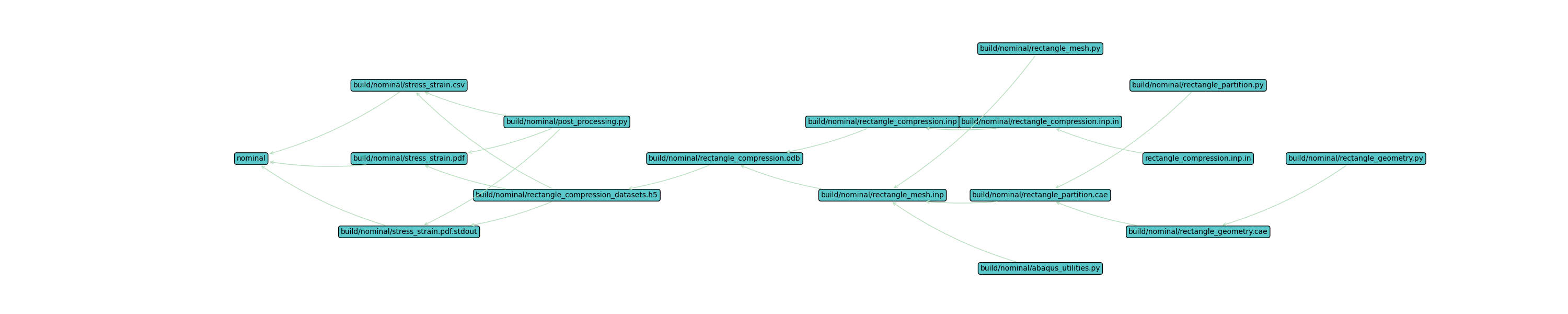
The workflow visualization should look similar to the image below, which is a representation of the directed graph constructed by SCons from the task definitions. The image starts with the final workflow target on the left, in this case the nominal simulation target alias. Moving left to right, the files required to complete the workflow are shown until we reach the original source file(s) on the far right of the image. The arrows represent actions and are drawn from a required source to the produced target. The Computational Practices introduction discusses the relationship of a Build System task and Directed graphs.

Quickstart

Contents

Quickstart#

Environment#

Directory Structure#

SConscript#

SConstruct#

Building targets#

Output Files#

Workflow Visualization#